Traffic Sign Classifier
Abstract
A traffic sign classifier is build using the LeNet-5 deep neural network topology. Given a dataset containing images from 43 distinct classes from the German Traffic Sign Dataset, a classifier is built that obtains a 93% classification accuracy on a holdout set. Class imbalances are addressed and corrected for, and an exploratory analysis of the dataset is performed.
Load The Data
import pickle

# load the database (already been pickled)

training_file =  "../../traffic-signs-data/train.p"
validation_file= "../../traffic-signs-data/valid.p"
testing_file =   "../../traffic-signs-data/test.p"

with open(training_file, mode='rb') as f:
    train = pickle.load(f)
with open(validation_file, mode='rb') as f:
    valid = pickle.load(f)
with open(testing_file, mode='rb') as f:
    test = pickle.load(f)

X_train, y_train = train['features'], train['labels']
X_valid, y_valid = valid['features'], valid['labels']
X_test, y_test = test['features'], test['labels']
Dataset Summary & Exploration
The pickled data is a dictionary with 4 key/value pairs:
-
'features'is a 4D array containing raw pixel data of the traffic sign images -
'labels'is a 1D array containing the label/class id of the traffic sign. The filesignnames.csvcontains id -> name mappings for each id. -
'sizes'is a list containing tuples, width, height, representing the original width and height the image. -
'coords'is a list containing tuples, (x1, y1, x2, y2) representing coordinates of a bounding box around the sign in the image. THESE COORDINATES ASSUME THE ORIGINAL IMAGE. THE PICKLED DATA CONTAINS RESIZED VERSIONS, 32x32, OF THESE IMAGES
Provide a Basic Summary of the Data Set
### Use numpy methods to output metadata
import numpy as np

# Number of training examples
n_train = train["labels"].shape

# Number of testing examples.
n_test = test["labels"].shape

# What's the shape of an traffic sign image?
# after resizing, train["sizes"] gives original shapes, which are different from one another
image_shape = train["features"][-1].shape

# How many unique classes/labels there are in the dataset?
n_classes = np.size(np.unique(train["labels"]))

print("Number of training examples =", n_train)
print("Number of testing examples =", n_test)
print("Number of validation examples = ", valid['labels'].shape)
print("Image data shape =", image_shape)
print("Number of classes =", n_classes)
Number of training examples = (34799,)
Number of testing examples = (12630,)
Number of validation examples =  (4410,)
Image data shape = (32, 32, 3)
Number of classes = 43
Exploratory visualization of the dataset
Some of what I think would be interesting would be frequency of class occurrence as a function of class. It’s important to identify class imbalances that could negatively affect classification accuracy.
### Data exploration visualization code goes here.
### Feel free to use as many code cells as needed.
import matplotlib.pyplot as plt
# Visualizations will be shown in the notebook.
%matplotlib inline
# plot class frequency
n, bins, patches = plt.hist(train["labels"], n_classes, normed=0, facecolor='green', alpha=0.75)
plt.xlabel('Class Label')
plt.ylabel('No. of Occurrences')
plt.title('Traffic Sign Instances Observed in Training Set')
plt.axis([0, 43, 0, 2100])

plt.show()
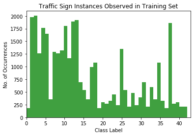
There is an apparent class imbalance…
Some classes are really underrepresented in the dataset, as can be seen from the histogram above. This will require some data augmentation. However, I don’t want to get into augmenting until after other preprocessing has been done (normalization, standardization, etc…).
# code adapted from https://github.com/netaz/carnd_traffic_sign_classifier
from skimage.color import gray2rgb
def plot_image(image, nr, nc, i, gray=False, xlabel="",ylabel=""):
    """
    If 'i' is greater than 0, then plot this image as
    a subplot of a larger plot.
    """

    if i>0:
        plt.subplot(nr, nc, i)
    else:
        plt.figure(figsize=(nr,nc))

    plt.xticks(())
    plt.yticks(())
    plt.xlabel(xlabel)
    if i % nc == 1:
        plt.ylabel(ylabel)
    plt.tight_layout()
    if gray:
        image_rgb = gray2rgb(image)
        image_rgb = image_rgb.transpose((2,0,1,3))
        image_rgb = image_rgb.reshape((32,32,3))
        plt.imshow(image_rgb, cmap="gray")
    else:
        plt.imshow(image)
pop_lbl = [2,10,14,25,37]
cnt = 0
for p,i in zip(pop_lbl,range(len(pop_lbl))):
    pop_idx = np.where(train["labels"]==p)
    for j in range(4):
        label = "class={}".format(str(pop_lbl[i]))
        plot_image(train["features"][pop_idx[0][j],:,:,:],len(pop_lbl),4,cnt+1,ylabel=label)
        cnt+=1
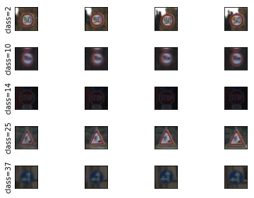
Some images are rather dark…
Images from classes 14 and 37 are very, very dark. Some preprocessing is apparently necessary to identify the features present in these images. More on this to come after the preprocessing section.
Design and Test a Model Architecture
Here is where I will build the classifier that learns to recognize traffic signs. I will train and test this model on the German Traffic Sign Dataset.
The LeNet-5 implementation is a solid point to start from. It’s predominately been used for handwritten digit recognition a la MNIST, however its topology allows for robust feature extraction on more complex image sets.
There are various aspects to consider when thinking about this problem:
- Neural network architecture (is the network over or underfitting?)
- Would preprocessing help; like normalization or colorspace conversion?
- Number of examples per label (some have more than others).
- Generate “fake” data. This will address class imbalances already found.
Preprocess the Dataset
# define a couple of helper functions to preprocess the images
# preprocessing will allow the network to perform more robust feature extraction

# Min-Max scaling for grayscale image data
# http://sebastianraschka.com/Articles/2014_about_feature_scaling.html#about-min-max-scaling
def normalize_scale(X):
    a = 0
    b = 1.0
    return a + X * (b-a) / 255

# http://lamda.nju.edu.cn/weixs/project/CNNTricks/CNNTricks.html
def standardize(X,test_set=False):
    if test_set:
        X -= np.mean(X_train)
        X /= np.std(X_train)
    else:
        X -= np.mean(X) # zero-center
        X /= np.std(X) # normalize
    return (X)

def rgb2gray(X):
    gray = np.dot(X, [0.299, 0.587, 0.114])
    gray = gray.reshape(len(X),32,32,1)
    return gray

# preprocessing pipeline
def preprocess_dataset(X,test_set=False):
    X = rgb2gray(X)
    X = normalize_scale(X)
    X = standardize(X,test_set)
    return X
X_train = preprocess_dataset(X_train)
X_valid = preprocess_dataset(X_valid)
X_test = preprocess_dataset(X_test)
pop_lbl = [14]
cnt = 0
for p,i in zip(pop_lbl,range(len(pop_lbl))):
    pop_idx = np.where(train["labels"]==p)
    for j in range(5):
        label = "class={}".format(str(pop_lbl[i]))
        plot_image(X_train[pop_idx[0][j],:,:,:],len(pop_lbl),5,cnt+1,gray=True,ylabel=label)
        cnt+=1
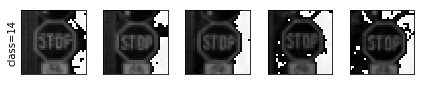
The features are more resolved with the preprocessing steps
The images are now much more resolved and easier to discern with the naked eye. Hopefully this will make the model’s classification accuracy higher.
Augmenting the dataset to rebalance
To augment the dataset, the following methods can be employed from the skimage.ndimage package. Images are rotated by some number of degrees, shifted by some number of pixels, or a combination of the two methods.
# first define some helper functions
def counts(label, y):
    """
    counts the number of instances of class in y
    """
    n_counts = y[y==label].shape[0]
    #print(n_counts)
    return n_counts

def class_images(label, X, y):
    """
    Return a list containing all of the images of class 'img_class',
    from dataset X
    """
    n_counts = counts(label, y)
    img_list = []
    cnt = 0
    while n_counts>0:
        if y[cnt] == label:
            image = X[i].squeeze()
            img_list.append(image)
            n_counts -= 1
        cnt += 1
    return img_list


from scipy import ndimage
import math
import random

def augment_class(class_images, class_to_augment, X, y, num):
    nimages = len(class_images)
    ncols = 10
    nrows = math.ceil(nimages/ncols)

    j = 0
    listX = []
    listy = []
    for _x,_y in zip(X, y):
        listX.append(_x)
        listy.append(_y)
    ops = ['rotate', 'shift', 'rotate-shift']
    for image,i in zip(class_images, range(nimages)):
        image = image.reshape((32,32,1))
        orig_img = image
        for n in range(num):
            op = random.choice(ops)
            if op=='rotate':
                image = ndimage.rotate(orig_img, random.randint(-15, 15), reshape=False)
            elif op=='shift':
                shift_size = random.randint(-5, 5)
                image = ndimage.shift(orig_img, (shift_size, shift_size,0), order=0) #'bilinear'
            elif op=='rotate-shift':
                image = ndimage.rotate(orig_img, random.randint(-15, 15), reshape=False)
                shift_size = random.randint(-5, 5)
                image = ndimage.shift(image, (shift_size, shift_size,0), order=0) #'bilinear'
            else:
                assert 0, 'unknown/unspecified augmentation operation'
            listX.append(image)
            listy.append(class_to_augment)

    return i, np.array(listX), np.array(listy)
classes_to_augment = [0,6,16,19,20,21,22,23,24,26,27,29,30,32,34,36,37,39,40,41,42]
for class_to_augment in classes_to_augment:
    images = class_images(class_to_augment, X=X_train, y=y_train)
    n_images, X_train, y_train = augment_class(images, class_to_augment, X=X_train, y=y_train, num=1)
    print("Done augmenting {} images to class {}".format(n_images, class_to_augment))
Done augmenting 179 images to class 0
Done augmenting 359 images to class 6
Done augmenting 359 images to class 16
Done augmenting 179 images to class 19
Done augmenting 299 images to class 20
Done augmenting 269 images to class 21
Done augmenting 329 images to class 22
Done augmenting 449 images to class 23
Done augmenting 239 images to class 24
Done augmenting 539 images to class 26
Done augmenting 209 images to class 27
Done augmenting 239 images to class 29
Done augmenting 389 images to class 30
Done augmenting 209 images to class 32
Done augmenting 359 images to class 34
Done augmenting 329 images to class 36
Done augmenting 179 images to class 37
Done augmenting 269 images to class 39
Done augmenting 299 images to class 40
Done augmenting 209 images to class 41
Done augmenting 209 images to class 42
# plot class frequency
n, bins, patches = plt.hist(y_train, n_classes, normed=0, facecolor='green', alpha=0.75)
plt.xlabel('Class Label')
plt.ylabel('No. of Occurrences')
plt.title('Traffic Sign Instances Observed in First Augmented Training Set')
plt.axis([0, 43, 0, 2100])

plt.show()
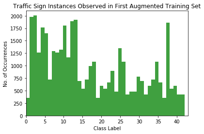
After the first augmentation, there still seem to be some imbalanced classes. Let’s go through another augmentation on the imbalanced classes.
classes_to_augment = [0,19,24,27,32,37,41,42]
for class_to_augment in classes_to_augment:
    images = class_images(class_to_augment, X=X_train, y=y_train)
    n_images, X_train, y_train = augment_class(images, class_to_augment, X=X_train, y=y_train, num=2)
    print("Done augmenting {} images to class {}".format(n_images, class_to_augment))

print("New training set size", len(X_train))
Done augmenting 359 images to class 0
Done augmenting 359 images to class 19
Done augmenting 479 images to class 24
Done augmenting 419 images to class 27
Done augmenting 419 images to class 32
Done augmenting 359 images to class 37
Done augmenting 419 images to class 41
Done augmenting 419 images to class 42
New training set size 47399
# plot class frequency
n, bins, patches = plt.hist(y_train, n_classes, normed=0, facecolor='green', alpha=0.75)
plt.xlabel('Class Label')
plt.ylabel('No. of Occurrences')
plt.title('Traffic Sign Instances Observed in Second Augmented Training Set')
plt.axis([0, 43, 0, 2100])

plt.show()
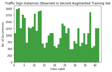
This is looking passable now…
There’s appears to be no worse than a 4:1 class imbalance now! This should be good enough to train on (or at least to try).
Model Architecture
import tensorflow as tf

from tensorflow.contrib.layers import flatten

def LeNet(x):
    # Arguments used for tf.truncated_normal, randomly defines variables for the weights and biases for each layer
    mu = 0
    sigma = 0.1

    # Layer 1: Convolutional. Input = 32x32x1. Output = 28x28x6.
    conv1_W = tf.Variable(tf.truncated_normal(shape=(5, 5, 1, 6), mean = mu, stddev = sigma))
    conv1_b = tf.Variable(tf.zeros(6))
    conv1   = tf.nn.conv2d(x, conv1_W, strides=[1, 1, 1, 1], padding='VALID') + conv1_b

    # Activation.
    conv1 = tf.nn.relu(conv1)

    # Pooling. Input = 28x28x6. Output = 14x14x6.
    conv1 = tf.nn.max_pool(conv1, ksize=[1, 2, 2, 1], strides=[1, 2, 2, 1], padding='VALID')

    # Layer 2: Convolutional. Output = 10x10x16.
    conv2_W = tf.Variable(tf.truncated_normal(shape=(5, 5, 6, 16), mean = mu, stddev = sigma))
    conv2_b = tf.Variable(tf.zeros(16))
    conv2   = tf.nn.conv2d(conv1, conv2_W, strides=[1, 1, 1, 1], padding='VALID') + conv2_b

    # Activation.
    conv2 = tf.nn.relu(conv2)

    # Pooling. Input = 10x10x16. Output = 5x5x16.
    conv2 = tf.nn.max_pool(conv2, ksize=[1, 2, 2, 1], strides=[1, 2, 2, 1], padding='VALID')

    # Flatten. Input = 5x5x16. Output = 400.
    fc0   = flatten(conv2)

    # Layer 3: Fully Connected. Input = 400. Output = 120.
    fc1_W = tf.Variable(tf.truncated_normal(shape=(400, 120), mean = mu, stddev = sigma))
    fc1_b = tf.Variable(tf.zeros(120))
    fc1   = tf.matmul(fc0, fc1_W) + fc1_b

    # Activation.
    fc1    = tf.nn.relu(fc1)

    # Layer 4: Fully Connected. Input = 120. Output = 84.
    fc2_W  = tf.Variable(tf.truncated_normal(shape=(120, 84), mean = mu, stddev = sigma))
    fc2_b  = tf.Variable(tf.zeros(84))
    fc2    = tf.matmul(fc1, fc2_W) + fc2_b

    # Activation.
    fc2    = tf.nn.relu(fc2)
    #fc2    = tf.nn.dropout(fc2, 0.5) # this actually hurt validation accuracy, maybe revisit?

    # Layer 5: Fully Connected. Input = 84. Output = 43.
    fc3_W  = tf.Variable(tf.truncated_normal(shape=(84, n_classes), mean = mu, stddev = sigma))
    fc3_b  = tf.Variable(tf.zeros(n_classes))
    logits = tf.matmul(fc2, fc3_W) + fc3_b

    return logits
Train, Validate and Test the Model
A validation set can be used to assess how well the model is performing. A low accuracy on the training and validation sets imply underfitting. A high accuracy on the training set but low accuracy on the validation set implies overfitting.
def evaluate(X_data, y_data):
    num_examples = len(X_data)
    total_accuracy = 0
    sess = tf.get_default_session()
    for offset in range(0, num_examples, BATCH_SIZE):
        batch_x, batch_y = X_data[offset:offset+BATCH_SIZE], y_data[offset:offset+BATCH_SIZE]
        accuracy = sess.run(accuracy_operation, feed_dict={x: batch_x, y: batch_y})
        total_accuracy += (accuracy * len(batch_x))
    return total_accuracy / num_examples
EPOCHS = 50
BATCH_SIZE = 128
x = tf.placeholder(tf.float32, (None, 32, 32, 1))
y = tf.placeholder(tf.int32, (None))
one_hot_y = tf.one_hot(y, n_classes)

rate = 0.001

logits = LeNet(x)
cross_entropy = tf.nn.softmax_cross_entropy_with_logits(logits=logits, labels=one_hot_y)
#cross_entropy = tf.contrib.losses.softmax_cross_entropy(logits, labels, weight=1.0, scope=None)
loss_operation = tf.reduce_mean(cross_entropy)
optimizer = tf.train.AdamOptimizer(learning_rate = rate)
training_operation = optimizer.minimize(loss_operation)

correct_prediction = tf.equal(tf.argmax(logits, 1), tf.argmax(one_hot_y, 1))
accuracy_operation = tf.reduce_mean(tf.cast(correct_prediction, tf.float32))
### THIS IS THE MAIN EXEC OF THE PROJECT
### The training set is used to compute the weights of the neural network and it's accuracy on each 10th epoch
### is reported
from sklearn.utils import shuffle
saver = tf.train.Saver()
with tf.Session() as sess:
    sess.run(tf.global_variables_initializer())
    num_examples = len(X_train)

    print("Training...")
    print()
    for i in range(EPOCHS):
        X_train, y_train = shuffle(X_train, y_train)
        for offset in range(0, num_examples, BATCH_SIZE):
            end = offset + BATCH_SIZE
            batch_x, batch_y = X_train[offset:end], y_train[offset:end]
            sess.run(training_operation, feed_dict={x: batch_x, y: batch_y})

        validation_accuracy = evaluate(X_valid, y_valid)
        if i % 10 == 0:
            print("EPOCH {} ...".format(i+1))
            print("Validation Accuracy = {:.3f}".format(validation_accuracy))
            print()
        elif i == EPOCHS-1:
            print("EPOCH {} ...".format(i+1))
            print("Validation Accuracy = {:.3f}".format(validation_accuracy))
            print()


    saver.save(sess, './lenet')
    print("Model saved")
Training...

EPOCH 1 ...
Validation Accuracy = 0.791

EPOCH 11 ...
Validation Accuracy = 0.902

EPOCH 21 ...
Validation Accuracy = 0.918

EPOCH 31 ...
Validation Accuracy = 0.929

EPOCH 41 ...
Validation Accuracy = 0.916

EPOCH 50 ...
Validation Accuracy = 0.932

Model saved
Test a Model on New Images
To give more insight into how the model works, let’s test five pictures of German traffic signs from the web and use the model to predict the traffic sign type. These images were not part of the original dataset, so we can get an idea of how good the classifier is on arbitrary German traffic signs, provided they are one of the classes in the dataset.
Load and Output the Images
Remember: the images must first be preprocessed to match the proper input to LeNet.
### Load the images and plot them here.
### Feel free to use as many code cells as needed.
from PIL import Image

img = np.zeros((5,32,32,3))
img[0,:,:,:] = np.array(Image.open('7501_Hoechstgeschwindigkeit_02.jpg').resize((32,32)))
img[1,:,:,:] = np.array(Image.open('7501_stop_01.jpg').resize((32,32)))
img[2,:,:,:] = np.array(Image.open('caution.jpg').resize((32,32)))
img[3,:,:,:] = np.array(Image.open('end_no_passing.jpg').resize((32,32)))
img[4,:,:,:] = np.array(Image.open('no_passing.jpg').resize((32,32)))

test_set = preprocess_dataset(img,True)
test_lbl = np.array([3,14,18,41,9])

for j in range(test_lbl.shape[0]):
    plot_image(test_set[j,:,:,:],1,5,j+1,gray=True)

Predict the Sign Type for Each Image
### Run the predictions here and use the model to output the prediction for each image.
new_saver = tf.train.import_meta_graph('lenet.meta')
with tf.Session() as sess:
    sess.run(tf.global_variables_initializer())
    new_saver.restore(sess, tf.train.latest_checkpoint('.'))
    output = sess.run(logits, feed_dict={x: test_set})
maxes = np.amax(output,axis=1)
cl = np.zeros((len(maxes)))
cnt = 0
for m,cnt in zip(maxes,range(len(maxes))):
    print("(Prediction, Actual) = ({},{})".format(np.where(output[cnt]>=maxes[cnt])[0][0], test_lbl[cnt]))
(Prediction, Actual) = (1,3)
(Prediction, Actual) = (25,14)
(Prediction, Actual) = (18,18)
(Prediction, Actual) = (41,41)
(Prediction, Actual) = (9,9)
Analyze Performance
As can be seen from the previous cell’s output, three of the five test were predicted correctly, giving an accuracy of 60%. This isn’t bad, considering that class 1 has a high number of instances and class 14 images are pretty dark in the dataset.
Output Top 5 Softmax Probabilities For Each Image Found on the Web
For each of the new images, print out the model’s softmax probabilities to show the certainty of the model’s predictions. tf.nn.top_k is a Tensorflow routine that outputs the top k probabilities.
The example below demonstrates how tf.nn.top_k can be used to find the top k predictions for each image.
tf.nn.top_k will return the values and indices (class ids) of the top k predictions. So if k=3, for each sign, it’ll return the 3 largest probabilities (out of a possible 43) and the correspoding class ids.
Take this numpy array as an example. The values in the array represent predictions. The array contains softmax probabilities for five candidate images with six possible classes. tk.nn.top_k is used to choose the three classes with the highest probability:
# (5, 6) array
a = np.array([[ 0.24879643,  0.07032244,  0.12641572,  0.34763842,  0.07893497,
         0.12789202],
       [ 0.28086119,  0.27569815,  0.08594638,  0.0178669 ,  0.18063401,
         0.15899337],
       [ 0.26076848,  0.23664738,  0.08020603,  0.07001922,  0.1134371 ,
         0.23892179],
       [ 0.11943333,  0.29198961,  0.02605103,  0.26234032,  0.1351348 ,
         0.16505091],
       [ 0.09561176,  0.34396535,  0.0643941 ,  0.16240774,  0.24206137,
         0.09155967]])
Running it through sess.run(tf.nn.top_k(tf.constant(a), k=3)) produces:
TopKV2(values=array([[ 0.34763842,  0.24879643,  0.12789202],
       [ 0.28086119,  0.27569815,  0.18063401],
       [ 0.26076848,  0.23892179,  0.23664738],
       [ 0.29198961,  0.26234032,  0.16505091],
       [ 0.34396535,  0.24206137,  0.16240774]]), indices=array([[3, 0, 5],
       [0, 1, 4],
       [0, 5, 1],
       [1, 3, 5],
       [1, 4, 3]], dtype=int32))
Looking just at the first row we get [ 0.34763842, 0.24879643, 0.12789202], you can confirm these are the 3 largest probabilities in a. You’ll also notice [3, 0, 5] are the corresponding indices.
### Print out the top five softmax probabilities for the predictions on the German traffic sign images found on the web.
with tf.Session() as sess:
    tops = sess.run(tf.nn.top_k(tf.nn.softmax(tf.constant(output)),k=5))
    print(tops)
TopKV2(values=array([[  1.00000000e+00,   5.76315484e-09,   1.25874606e-11,
          2.02269581e-12,   4.36664585e-15],
       [  9.89064455e-01,   9.48491786e-03,   5.03997027e-04,
          3.41146340e-04,   1.84364195e-04],
       [  1.00000000e+00,   7.57849783e-10,   3.18966655e-14,
          4.15005825e-15,   1.16327667e-16],
       [  9.99906659e-01,   5.87343457e-05,   1.69039595e-05,
          8.05835862e-06,   5.43485476e-06],
       [  9.91937459e-01,   5.52976551e-03,   2.06296914e-03,
          2.69575568e-04,   9.10933668e-05]], dtype=float32), indices=array([[ 1,  6,  2, 31, 32],
       [25, 24, 28, 29, 18],
       [18, 26, 27, 28, 20],
       [41, 32,  6, 42, 36],
       [ 9, 17, 41, 20, 16]], dtype=int32))
Just out of curiosity…
There is a test set provided, how does the model perform on it?
new_saver = tf.train.import_meta_graph('lenet.meta')
with tf.Session() as sess:
    sess.run(tf.global_variables_initializer())
    new_saver.restore(sess, tf.train.latest_checkpoint('.'))
    test_accuracy = evaluate(X_test, y_test)
    print("Test Accuracy = {:.3f}".format(test_accuracy))
Test Accuracy = 0.922
Visualize the Neural Network’s State with Test Images
After successfully training a neural network you can see what its feature maps look like by plotting the output of the network’s weight layers in response to a test stimuli image. From these plotted feature maps, it’s possible to see what characteristics of an image the network finds interesting. For a sign, maybe the inner network feature maps react with high activation to the sign’s boundary outline or to the contrast in the sign’s painted symbol.
For an example of what feature map outputs look like, you could check out NVIDIA’s results in their paper End-to-End Deep Learning for Self-Driving Cars in the section Visualization of Internal CNN State. NVIDIA was able to show that their network’s inner weights had high activations to road boundary lines by comparing feature maps from an image with a clear path to one without.
### Visualize the network's feature maps here.

# image_input: the test image being fed into the network to produce the feature maps
# tf_activation: should be a tf variable name used during your training procedure that represents the calculated state of a specific weight layer
# activation_min/max: can be used to view the activation contrast in more detail, by default matplot sets min and max to the actual min and max values of the output
# plt_num: used to plot out multiple different weight feature map sets on the same block, just extend the plt number for each new feature map entry

def outputFeatureMap(image_input, tf_activation, activation_min=-1, activation_max=-1 ,plt_num=1):
    # Here make sure to preprocess the image_input in a way the network expects
    # Note: x should be the same name as your network's tensorflow data placeholder variable
    # If you get an error tf_activation is not defined it maybe having trouble accessing the variable from inside a function
    activation = tf_activation.eval(session=sess,feed_dict={x : image_input})
    featuremaps = activation.shape[3]
    plt.figure(plt_num, figsize=(15,15))
    for featuremap in range(featuremaps):
        plt.subplot(6,4, featuremap+1) # sets the number of feature maps to show on each row and column
        plt.title('FeatureMap ' + str(featuremap)) # displays the feature map number
        if activation_min != -1 & activation_max != -1:
            plt.imshow(activation[0,:,:, featuremap], interpolation="nearest", vmin =activation_min, vmax=activation_max, cmap="gray")
        elif activation_max != -1:
            plt.imshow(activation[0,:,:, featuremap], interpolation="nearest", vmax=activation_max, cmap="gray")
        elif activation_min !=-1:
            plt.imshow(activation[0,:,:, featuremap], interpolation="nearest", vmin=activation_min, cmap="gray")
        else:
            plt.imshow(activation[0,:,:, featuremap], interpolation="nearest", cmap="gray")
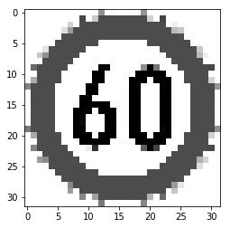
img = np.zeros((1,32,32,3))
img[0,:,:,:] = np.array(Image.open('7501_Hoechstgeschwindigkeit_02.jpg').resize((32,32)))
image_input = preprocess_dataset(img, True)
with tf.Session() as sess:
    new_saver = tf.train.import_meta_graph('lenet.meta')
    new_saver.restore(sess, tf.train.latest_checkpoint('.'))

    conv_1 = tf.get_default_graph().get_tensor_by_name("Conv2D_1:0")

    plt.imshow(np.squeeze(image_input),cmap='gray')
    plt.show()
    outputFeatureMap(image_input, conv_1)
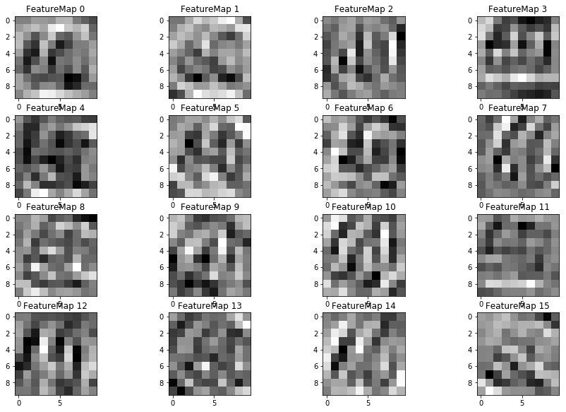
Any layer in the network could be used to identify which features were most important to that layer. From this, the user can see that neural networks aren’t merely a “black box”; each layer refines a greater level of detail than the one previous.