Unscented Kalman Filters
Sample Estimation Problem
A coworker approached me sometime back asking me to address a state estimation problem he was having. So, I whipped up this notebook in my free time to address the problem. By ‘tag’, I mean AprilTags, the set of markers for fiducial landmarking.
Preamble
You are able to measure the distance to the tag, but you are uncertain of the rotation angle and of the minimum distance to the tag, which occurs when the camera is aligned with the tag.
First, a few definitions will help
\[\mathbf{x} = \begin{pmatrix} \beta \\ \psi \end{pmatrix}\]$\mathbf{x}$ is the state vector we want to estimate; $\beta$ is the minimum distance to the tag and $\psi$ is the angle of robot rotation relative to the tag.
The general form of the problem I am considering is the estimation problem:
\[\dot{\mathbf{x}} = \mathbf{f}(\mathbf{x}) + \mathbf{g}(\mathbf{u}) + \mathbf{v} \\ \mathbf{z} = \mathbf{h}(\mathbf{x}) + \mathbf{w},\]where $\mathbf{u}$ is the control vector. In this case, I assume we are able to command velocity and $\dot{\psi}$. The variables $\mathbf{v},\mathbf{w}$ are process and measurement noise vectors, respectively.
I don’t know much about the intricacies of the problem, so I’ll assume that the system is as simple as possible; that is, the robot is not moving and is spinning at a constant rate. The measurement is the distance of a fixed-body camera to the tag. I drop the bold font since our measurement is only one-dimensional:
\[h(\mathbf{x}) = \sqrt{(\beta+r)^2 + 1 - 2(\beta+r)r \cos\psi},\]where $r$ is the robot’s radius.
Implementation in Python
I really hate having to compute Jacobians, so I decided to use an unscented Kalman filter here to avoid such nonsense. There’s a nice implementation in Python called filterpy that I was able to install and run really quickly. Here’s the solution:
import numpy as np
from filterpy.kalman import UnscentedKalmanFilter
from filterpy.kalman import JulierSigmaPoints
import matplotlib.pyplot as plt
First, define the ground truth:
beta      = 1.;
psi_start =  np.pi / 4.
psi_end   = -np.pi / 4.
psi_rate  = -0.2
psi       = psi_start
dt        = .01
r         = .4
Define the functions needed to do the prediction and measurement updates:
def fx(x,dt,psi_rate=-0.2):
    x[1] += psi_rate * dt
    return x

def hx(x,r=0.4):
    bpr  = x[0]+r
    bpr2 = bpr * bpr
    return np.sqrt(bpr2 + 1. - 2. * bpr * r * np.cos(x[1]))
Initialize the UKF:
dim_x = 2
dim_z = 1

points = JulierSigmaPoints(n=dim_x, kappa=3.-dim_x, sqrt_method=np.linalg.cholesky)

ukf = UnscentedKalmanFilter(dim_x=dim_x, dim_z=dim_z, dt=dt, fx=fx, hx=hx, points=points, sqrt_fn=np.linalg.cholesky)
"""
 initialize state and covariance
"""
beta_worst = .9
psi_worst = .9
ukf.x = np.array([beta_worst,psi_worst])
# you will probably want to change the noise terms to something more appropriate
beta_1sig = .02 # 2 cm
psi_1sig = np.pi/180. # 1 deg
ukf.Q = np.zeros((2,2))
ukf.Q[0,0] = beta_1sig * beta_1sig
ukf.Q[1,1] = psi_1sig * psi_1sig
ukf.P = 1000*ukf.Q # set to something arbitrarily large to monitor filter convergence
d_1sig = .02
ukf.R = d_1sig * d_1sig
Now, actually run the simulation:
# create containers for plotting (initialized to initial condition)
x_t = []
d   = []
d_p = []
d_t = []
x_e = []
P_e = []

while psi > -np.pi/4:
    # get truth
    psi += psi_rate * dt
    x_c = [beta,psi]
    x_t.append(x_c)

    # predict
    ukf.predict(fx_args=psi_rate)

    # get measurement
    d_c = hx(x_c,r=r)
    d_t.append(d_c)
    d_m = d_c + np.random.normal(0.,d_1sig,1)
    d_p.append( hx(ukf.x,r=r) )
    d.append(d_m)

    # update kalman filter
    ukf.update(np.array(d_m),hx_args=r)

    # store states
    x_e.append([ukf.x[0],ukf.x[1]])
    P_e.append([ukf.P[0,0],ukf.P[1,1]])
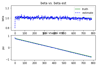
Now, plot the output:
# create numpy containers for plotting
xnp_t = np.array(x_t).reshape((len(x_t),2))
xnp_e = np.array(x_e).reshape((len(x_e),2))
Pnp_e = np.array(P_e).reshape((len(P_e),2))

plt.figure()
plt.subplot(2,1,1)
plt.plot(xnp_t[:,0],'g', label="truth")
plt.plot(xnp_e[:,0],'b--', label="estimate")
plt.legend(loc='best')
plt.title("beta vs. beta est")
plt.ylabel("beta")
plt.ylim((0.75,1.25))

plt.subplot(2,1,2)
plt.plot(xnp_t[:,1],'g')
plt.plot(xnp_e[:,1],'b--')
plt.title("psi vs. psi est")
plt.ylabel("psi")
plt.ylim((-np.pi/3.,np.pi/3.))
plt.show()

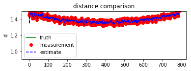
# now do the distance
dnp_t = np.array(d_t)
dnp_m = np.array(d)
dnp_e = np.array(d_p)

plt.figure()
plt.subplot(2,1,1)
plt.plot(dnp_t,'g', label="truth")
plt.plot(dnp_m,'ro', label="measurement")
plt.plot(dnp_e,'b--', label="estimate")
plt.legend(loc='best')
plt.title("distance comparison")
plt.ylabel("d")
plt.ylim((.9,1.5))
plt.show()

Comments
- The estimate is still pretty noisy, indicating an improper tuning of process noise