Simple Gaussian Optimization
Motivating Remarks
I have recently been butting my head against my desk in frustration at a noise model I have been using. The system I have been developing appears very sensitive to this noise distribution and I have been having difficulty finding a good set of parameters to give me good performance. This got me thinking about how I could setup a way to find the best estimate of these parameters, which led me to an approach that I outline here.
I have posted the Jupyter notebook if you want to fork it and play around with it for yourself. Maybe you will get something useful out of using this approach. I know that I have. Thanks for reading!
Introduction
When trying to estimate a quantity with uncertainty, the first question is usually: what is the best way to estimate the uncertainty? I will address this question in this notebook.
Let’s say that, either through some prior knowledge or justification, that we know, on average, where we expect the the quantity to be and that the underlying process is drawn from a normal distribution. Are these assumptions justified? Well, this depends entirely upon the problem. However, in practice, Gaussian distributed noise is used extensively because there are closed-form solutions for optimal estimates with Gaussian uncertainty, e.g. the Kalman filter. Also, because of the Central Limit Theorem, the sum of independent random variables tends towards a Gaussian distribution.
For simplicity, I will consider the one-dimensional case with zero mean, but the method will generalize to higher dimensions and for non-zero means. Let’s start with a set of 100 points.
import numpy as np
import matplotlib.pyplot as plt
# initialize random number seed (for repeatability)
np.random.seed(seed=0)
# feel free to play around with these
sigma_act = 2.179
N = 100
# create sample points
samples = sigma_act*np.random.randn(100,1)
fig, ax = plt.subplots(1,1)
ax.scatter(samples, np.zeros_like(samples))
ax.set_xlabel('value')
ax.set_ylabel('unused')
ax.set_title('Scatterplot to show grouping of points')
plt.show()
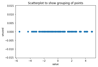
We can see there is the greatest density of points near 0, and that this density gets smaller as the distance from zero gets bigger. We’ve decided on trying to fit a Gaussian to this, so how can we find the best Gaussian? We can use the notion of likelihood. The best fit should be the most likely one. The li kelihood function for Gaussians is a smooth, positive-definite function with a single peak at the mean value. This fact makes our fitting problem amenable to solution via optimization: We can start with some initial guess and then iteratively move towards the best one.
In practice, maximizing likelihood is best achieved by looking at the related log-likelihood, which is the natural log of the likelihood function. This is done, particularly in higher-dimensional problems, because the likelihood function can involve raising $e$ to very small powers: \(<-200\), or smaller. This would wreak havoc on any numerical scheme!
Let’s see if we can use scipy to find our best fit for us.
Optimization Method
Scipy has a slew of optimization methods; each of which requires a function definition, which we have already, and an initial guess, which we don’t. Let’s start with the assumption that our uncertainty is really small; i.e. we know with high confidence where our unknown quantity will be.
from scipy.stats import norm  # for plotting gaussian pdf

# make our initial guess *really* poor - recall definition of sigma_act = 2.179 above
sigma_guess = 0.1

fig, ax = plt.subplots(1,1)
x = np.linspace(-5*sigma_act, 5*sigma_act, 100)
# plot our samples again
ax.scatter(samples, np.zeros_like(samples))
# plot our candidate gaussian fit
ax.plot(x, norm.pdf(x, loc=0, scale=sigma_guess), 'r--', label='guess')
ax.set_xlabel('value')
ax.set_ylabel('pdf')
ax.set_title('Our initial fit is very poor')
plt.legend()
plt.show()
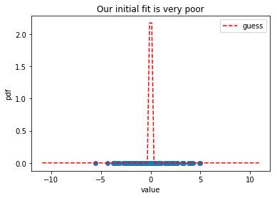
As you can see, our initial guess is very bad: there are data points that are well outside of the dashed red line. Can we make this estimate better by improving our guess iteratively? Let’s use scipy to find out.
from scipy.optimize import minimize
def neg_log_lhood(s, x):
# zero mean
# add the "-" sign because we want to maximize but are using the minimize method
return -(-0.5 * len(x) * np.log(2*np.pi*s**2) - 1./(2.*s**2)*sum([xx**2 for xx in x]))
def grad(s, x):
# perform a central difference numerical derivative with h = 1e-8
return (neg_log_lhood(s+1e-8, x) - neg_log_lhood(s-1e-8, x)) / (2e-8)
# scipy's minimize method returns a solution struct, which contains the solution (if one was found)
# and a message (and other things, check the docs)
sol = minimize(log_lhood, sigma_guess, args=(samples), jac=grad, method='bfgs')
print(sol.message)
if sol.success:
print('sigma_final = {}'.format(sol.x[0]))
print('log_lhood(sigma_final) = {} in {} iterations'.format(-neg_log_lhood(sol.x[0], samples)[0], sol.nit))
else:
print('No solution found')
fig, ax = plt.subplots(1,1)
# plot our samples again
ax.scatter(samples, np.zeros_like(samples))
ax.plot(x, norm.pdf(x, loc=0, scale=sol.x), 'k--', label='optimal')
ax.set_xlabel('value')
ax.set_ylabel('pdf')
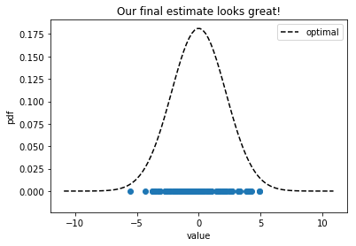
ax.set_title('Our final estimate looks great!')
plt.legend()
plt.show()
Optimization terminated successfully.
sigma_final = 2.200038675142532
log_lhood(sigma_final) = -220.74134731683375 in 12 iterations
Closing Remarks
The initial distribution that we sampled our points from had $\sigma = 2.179$ and our final guess was $\sigma’ = 2.200$, which is pretty good. We went from having a relative error of over 90% and ended with about 1%. This is a canned example, but it illustrates an interesting point about parameter estimation in uncertainty quantification, namely that a global optimization scheme can be used to find the best Gaussian fit to set of data points.