Smooth Path Planning - overlaying a velocity profile
Introduction
This post extends work discussed previously. In that post, I presented a method for constructing geometrically-continuous paths up to third-order. I will now discuss how to take that path and build a trajectory that drives along it. The notion of “drives” is important here: trajectory motion is assumed tangent to the path. This restriction refers to car-like robots that, under normal conditions, point their front-end in the direction of motion.
In this context, “trajectory” means a time-series of pose data, \((x,y,\theta)\), along with controls, \((v,\omega)\), that define a motion profile for a differential-drive robot. Importantly, the method that I discuss here can be applied to any underlying path geometry, not just \(\eta^3\)-splines.
Before going into the method, I will outline some constraints that are imposed to make the problem tractable:
- Trajectories have fixed initial condition. The robot begins at known velocity \(v_0 \le v_{max}\) and acceleration \(a_0 \le a_{max}\), where \(v_{max}, a_{max}\) are the maximum velocity and acceleration, respectively.
- Trajectories must terminate with zero velocity and acceleration. This makes sense, because most objectives involve getting to some particular waypoint before being assigned a new task/action.
- Kinematic limits must be obeyed everywhere along the trajectory. These limits are on velocity, acceleration, and jerk.
- The kinematic limits are symmetric: \(*_{min} = -*_{max}\).
- The maximum velocity may need to be reduced to accommodate the other two constraints. It may not be feasible to reach the desired maximum velocity given the length of the underlying path and the maximum acceleration and jerk limits.
The Method
The method I propose here is homespun in that I have not found many resources that approach the problem in a similar way. In a nutshell, the robot begins by applying the maximum jerk, \(j_{max}\), until the maximum acceleration is reached. Once maximum acceleration has been achieved, the robot will continue accelerating until the time when minimum jerk, \(j_{min} = -j_{max}\), needs to be applied to smoothly transition from acceleration to maximum speed with zero acceleration. At this point, if there is enough path length to do so, the robot will cruise at the maximum speed \(v_{max}\). Otherwise, the robot will continue applying minimum jerk until maximum deceleration has been achieved. Deceleration at maximum rate continues until the time when the robot needs to apply maximum jerk to finish at zero velocity and zero acceleration.
Before going through each section in more detail, a kinematic assessment needs to be made regarding whether or not the maximum velocity can be achieved given the other limits and the path given. This analysis requires a shooting method, of sorts, where a trajectory starting at the given initial conditions is shot forwards in time and a trajectory starting from the desired terminal condition is shot backwards in time. The terminal point in time of each trajectory is when it reaches the desired velocity \(v_{max}\). The intersection of the two trajectories is then analyzed based upon the sum of the two trajectory lengths. If this sum is greater than the total path length, then the desired maximum velocity, \(v_{max}\) cannot be achieved and the maximum velocity must be adjusted, \(v'_{max} < v_{max}\). Otherwise, \(v'_{max} = v_{max}\) and there will be some amount of cruising time; time where the robot moves at \(v'_{max}\).
For details of how this analysis is done in practice, please see the implementation.
I’ll now go through the math for each section.
Section 1: Maximum jerk, part 1
The robot starts at $v = v_0$ and $a=a_0$. The amount of time needed to get to maximum acceleration from the initial acceleration $a_0$ is:
\[\begin{eqnarray} \Delta a &=& a_{max} - a_0 \\ \Delta t &=& \frac{\Delta a}{j_{max}} \end{eqnarray}\]Let $s_{s_1}$ denote the path length traversed by the robot while applying maximum jerk:
\[\begin{eqnarray} s_{s_1} &=& v_0 \Delta t + \frac{1}{2} a_0 \Delta t^2 + \frac{1}{6} j_{max} \Delta t^3. \\ v_{s_1} &=& v_0 + \frac{1}{2} j_{max} \Delta t^2 \end{eqnarray}\]Section 2: Maximum acceleration
The robot continues at maximum acceleration until it needs to begin slowing down to hit $v_{max}$. The time-of-traversal for this second section is:
\[\begin{eqnarray} v_f &\equiv& v'_{max} - \frac{a_{max}^2}{2 j_{max}} \\ \Delta v &=& v_f - v_{s_1} \\ \Delta t &=& \frac{\Delta v}{a_{max}} \end{eqnarray}\]Let $s_{s_2}$ denote the path length traversed by the robot while applying maximum acceleration:
\[\begin{eqnarray} s_{s_2} &=& v_{s_1} \Delta t + \frac{1}{2} a_{max} \Delta t^2 \\ v_{s_2} &=& v_{s_1} + a_{max} \Delta t. \end{eqnarray}\]Section 3: Minimum jerk, part 1
In order to obey the jerk limits, the robot must apply minimum jerk to take out all of the acceleration.
\[\begin{eqnarray} \Delta a &=& 0 - a_{max} = -a_{max} \\ \Delta t &=& \frac{-a_{max}}{j_{min}} = \frac{a_{max}}{j_{max}} \end{eqnarray}\]Let $s_{s_3}$ denote the path length traversed by the robot while applying minimum jerk:
\[\begin{eqnarray} s_{s_3} &=& v_{s_2} \Delta t + \frac{1}{6} j_{min} \Delta t^3 \\ v_{s_3} &=& v_{s_2} + \frac{1}{2} j_{min} \Delta t^2. \end{eqnarray}\]Section 4: Cruise, initial consideration.
If the initial analysis showed that there was remaining path after doing the shooting method discussed, then there will be a cruise section. The math of the cruise section is the easiest because there is no velocity change. Logically, it makes the most sense to consider this segment last, because we will take whatever unaccounted-for length and apply it as a cruise section.
Section 5: Minimum jerk, part 2
At the end of the cruise section, or the end of the first minimum jerk section if there is no cruise section, apply minimum jerk again until max deceleration is reached.
\[\begin{eqnarray} \Delta a &=& a_{min} - 0 = -a_{max} \\ \Delta t &=& \frac{-a_{max}}{j_{min}} = \frac{a_{max}}{j_{max}} \end{eqnarray}\]Let $s_{s_3}$ denote the path length traversed by the robot while again applying minimum jerk:
\[\begin{eqnarray} s_{s_5} &=& v'_{max} \Delta t + \frac{1}{6} j_{min} \Delta t^3 \\ v_{s_5} &=& v'_{max} + \frac{1}{2} j_{min} \Delta t^2. \end{eqnarray}\]Section 6: Minimum acceleration
The robot will continue decelerating at \(a_{min}\) until the time when it needs to apply maximum jerk to hit the terminal constraint of zero velocity and acceleration.
\[\begin{eqnarray} \Delta v &=& v_{s_5} - \frac{a_{min}^2}{2 j_{max}} \\ \Delta t &=& \frac{\Delta v}{a_{max}} \end{eqnarray}\]Let $s_{s_6}$ denote the path length traversed by the robot while applying minimum acceleration:
\[\begin{eqnarray} s_{s_6} &=& v_{s_5} \Delta t + \frac{1}{2} a_{min} \Delta t^2 \\ v_{s_6} &=& v_{s_5} + a_{min} \Delta t. \end{eqnarray}\]Section 7: Maximum jerk, part 2
Finally, to come to a stop at zero velocity we again apply maximum jerk. \(\begin{eqnarray} \Delta a &=& 0-a_{min} = a_{max} \\ \Delta t &=& \frac{\Delta a}{j_{max}} \end{eqnarray}\)
Let $s_{s_7}$ denote the path length traversed by the robot while again applying maximum jerk:
\[\begin{eqnarray} s_{s_7} &=& v_{s_6} \Delta t - \frac{1}{6} j_{max} \Delta t^3. \\ v_{s_7} &=& v_{s_6} - \frac{1}{2} j_{max} \Delta t^2 \end{eqnarray}\]Section 4: Cruise, final consideration
At this point, we have everything we need to determine how long of a section we will be able to cruise along at \(v'_{max}\). Upon construction of the path, we computed a total segment length, \(s_{tot}\), from which we will now subtract all of the computed segment lengths thus far:
\[\begin{eqnarray} s_{s_4} &=& s_{tot} - \sum_{i \neq 4} s_{s_i} \\ \Delta t &=& \frac{v'_{max}}{s_{s_4}}, \end{eqnarray}\]where, again, \(\Delta t\) is the time-of-traversal.
Implementation Details
Finding the point along the curve at a given time/velocity
Recall that paths are typically composed of segments stitched together, each one of which is parametrized by a continuous parameter \(u \in [0, 1]\). Now that we are trying to overlay a velocity profile on top of these path segments, we need to be careful to correctly map our current point, as constructed by our integrated velocity profile, \(s(t) = \int_0^t v(\tau) d \tau\), to the corresponding \(u\) on the current path. The objective, stated mathematically, is:
For any \(t \in [0, T]\), \(T\) is the final trajectory time, find the \(u\) along the path such that \(\begin{equation} s(u) \equiv \int_0^{u} \dot s(\tau) d \tau = \int_0^t v(\tau) d \tau \end{equation}\) given a velocity profile that also parametrizes the path. \(\dot s(\tau) \equiv \sqrt{\dot x(\tau)^2 + \dot y(\tau)^2}\).
This problem is solved using the Fundamental Theorem of Calculus, part 1 together with a Newton iteration scheme. The basic idea is that the two methods are used together to find the root of the nonlinear equation:
\[\begin{equation} f(u) = \int_0^u \dot s(\tau) d \tau - \int_0^t v(t) dt, \end{equation}\]where \(t, v(t)\) are known and \(s(\tau)\) is constructed during the initial path building step.
Application
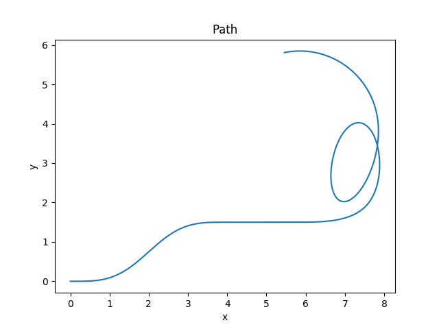
I begin with the path constructed in the previous post:
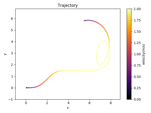
Now, I apply kinematic limits of \((v_{max}, a_{max}, j_{max}) = (2, 0.5, 1)\), where all units are SI. The resulting trajectory, represented as a colormap, is:
The velocity profiles, shown on one chart with two \(y\)-axes, is:
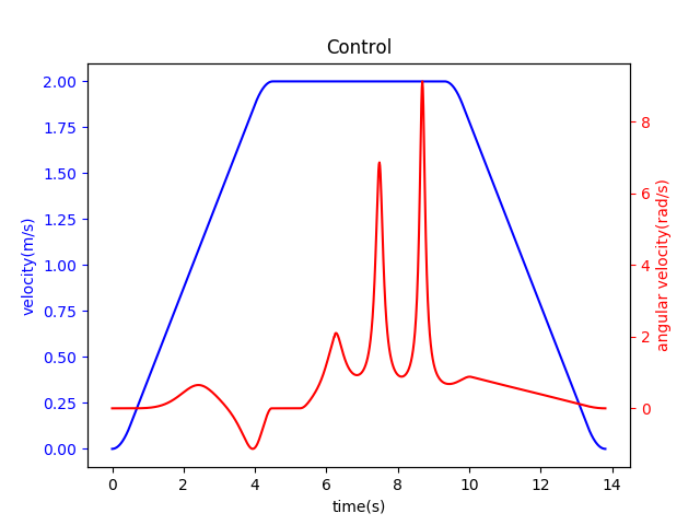
As expected, given the work on the path planner, the angular velocity is continuous. For most applications, this is very important, as the angular velocity can lead to wheel slip, instability, or other undesirable effects.
Concluding Remarks
A way of overlaying a velocity profile over a segments connecting multiple waypoints was presented. The velocity profile constructed obeys kinematic limits for maximum velocity, acceleration, and jerk. The angular velocity signal was shown to be continuous, which reinforces the idea continuous curvature presented in the \(\eta^3\) spline path planner. This mini-project was interesting and fun to work on. I hope that you, the interested reader, will find something worthwhile in either this post or my work supporting it. Cheers!