Introduction

I am currently enrolled in the OpenCV course “Computer Vision II: Applications (C++)”. For the second project, I had to create an application that would detect faces in a test image and then find the celebrities (from a provided dataset) whose faces most closely resemble those found in the test image. I put the phrase “most closely” in italics because I will discuss a few different approaches to finding the best match. To give a pictorial expression of the project’s objective, the course moderators provided the following expected output for two provided test images:

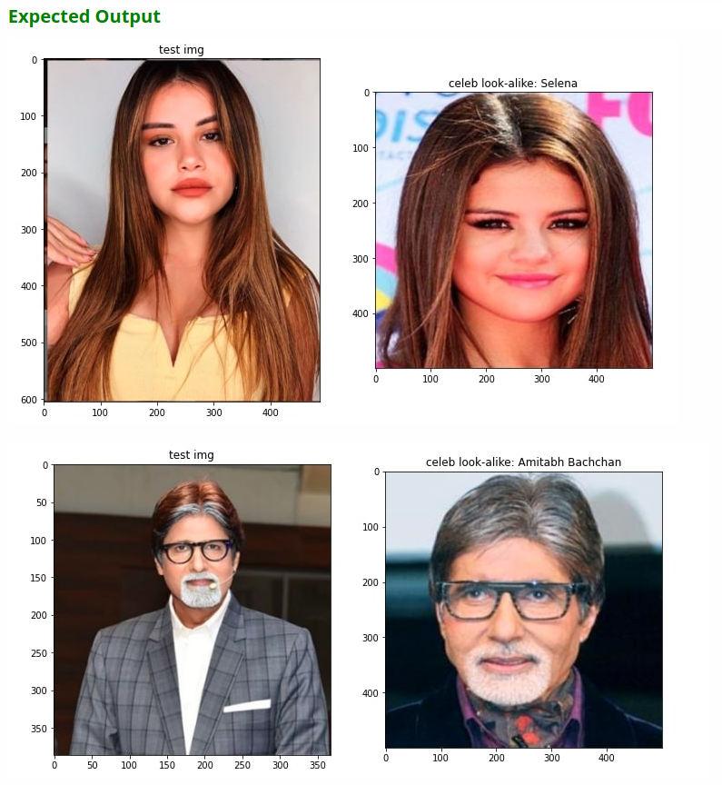
Note: the celebrity lookalike found for the top test image is displayed as Selena, however the lookalike image actually displayed is Selena Gomez. In the provided dataset, there are folders for both Selena and Selena Gomez, who are in fact two different people, but all images in both folders are for Selena Gomez.

In this blog post, I present a formal writeup of my solution addressing requirements of the project. Where appropriate, I will provide source code snippets highlighting important aspects of my approach.

Writeup

Objective

I will formally state the objective for the project here:

Given a dataset of celebrity images, labeled by name, create a low-dimensional descriptor representing the likeness of the face detected in each image. Using this low-dimensional descriptor, compute a similarity score between faces detected in test images and the celebrities in the dataset. The celebrity with the highest similarity score is declared the “lookalike” or “doppelganger” to an individual detected in a test image.

Dataset

The course moderators provided a dataset, dubbed “celeb_mini”, that contains ~5 images per celebrity for 1000+ celebrities. There is significant variation in the dataset across the following factors:

• Illumination
• Face pose
• Foreground clutter - some images have copyright data overlaid
• Sharpness/clarity of the image - some images are quite blurry

Solution

Because I am provided with a dataset for this activity, my solution has two phases: training and testing. During the training phase, I will find representative and informative descriptors for each image in the training set (i.e. the celeb_mini dataset). During the testing phase, I will apply the learned descriptor model (a function of the input image) to a test image and then find the most similar images in the training set with respect to the learned descriptor.

The solution is constructed in C++, and the primary APIs used in my solution are:

• OpenCV - used for basic image loading/saving and image processing
• dlib - used for linear algebra operations (length, linear systems solvers, and matrix processing), face detection, and for deep neural network inference
• matplotlibcpp - for plotting data

Before discussing each phase in greater detail, I will present my chosen descriptor model and justification.

Descriptor

Considering the givens and assumptions for this project, I’d like a descriptor with the following qualities:

• Low dimensionality (makes comparison simpler and reduces redundancy across dataset)
• Descriptors for images with the same label (i.e. represent the same celebrity) are highly similar (close in some metric sense)
• Descriptors for images with different labels are highly dissimilar (far apart in some metric sense)

In the course materials, a solution based on this representative example is presented that addresses all three points above using a deep learning-based approach. The solution uses a backbone architecture based on a ResNet pre-trained using metric loss to create a 128-dimensional descriptor of each input image. To avoid unnecessary effort in retraining the backbone network, I first wanted to see the performance on the assigned task (i.e. finding the correct lookalike for each of the two test images discussed in the Introduction section of this page) using the pre-trained network.

For the purpose of this project, this approach was found to be sufficient. In the Discussion section below, I will address deficiencies of using the pre-trained approach when considering use-cases outside of the defined boundaries for the project.

Training

This phase is not “training” in the typical sense, since a pre-trained network is used; rather it is more about generating descriptors for the images in the dataset using the pre-trained network. With this in mind, the training process is outlined as follows:

• Load training images
• Assign unique integral label to each subfolder in the dataset - images in each subfolder represent the same celebrity
• Map each folder to celebrity name - this will be used to assign celebrity name at the end of the testing process
• Load pre-trained model weights and biases for computing the descriptors
• for each image in the training image set
  • detect faces in image
  • for each face in detected faces
    • detect facial landmarks
    • use landmarks to crop facial region from image
    • compute descriptor using cropped facial region
• write celebrity name-to-label map to csv file - this will be used to match test image faces to celebrity likeness during the testing phase
• write descriptors, along with labels, to csv file for use during testing phase

The codebase for this step was built using materials provided by the course moderators, so I am not willing to share it here.

Testing

This phase’s primary concern is finding the celebrity that most closely resembles individuals detected in a test image. The process is outlined as follows:

• Load pre-trained model weights and biases (the same as in Training phase)
• Load csv file with celebrity name-to-label mapping
• Load csv file with descriptors and associated labels
• Load test image
• Detect faces in test image
• for each face in detected faces
  • detect facial landmarks
  • use landmarks to crop facial region from image
  • compute descriptor using cropped facial region
  • find most similar celebrity using loaded descriptors

The steps in the loop defined above should look familiar: they are the same as those used in the Training phase, with the addition of the matching step. The majority of original work that I did for this project was concerned with the calculation of a similarity metric, so I will focus the discussion around these points.

There are two metrics I used for computing similarity. The first is a simple, nearest-neighbor approach based on the Euclidean distance between descriptor vectors. The second uses Mahalanobis distance, which is a distance measure that is normalized by the covariance over samples from the training set with common label. I will now discuss these two approaches separately.

Euclidean distance

Euclidean distance is really easy to interpret: if I look at the descriptor vectors as embeddings in a 128D vector space, then similar vectors are ones whose tails are close to one another in the normal linear sense. In the context of the problem at-hand, the most similar celebrity to a person detected in a test image will have descriptor with shortest length to the descriptor representing the person detected in the test image.

The code to identify the top matches using a Euclidean distance metric is:

/**!
 * findKNearestNeighbors
 *
 * given an input descriptor and database of labeled descriptors, find the
 * top K best matches based using a Euclidean distance metric
 *
 */
bool findKNearestNeighbors(dlib::matrix<float, 0, 1> const& faceDescriptorQuery,
    std::vector<dlib::matrix<float, 0, 1>> const& faceDescriptors,
    std::vector<int> const& faceLabels, int const& k,
    std::vector<std::pair<int, double>>& matches) {
  // check that input vector sizes match, mark failure and exit if they don't
  if (faceLabels.size() != faceDescriptors.size()) {
    std::cout << "Size mismatch.  Exiting" << std::endl;
    return false;
  }

  // loop over all descriptors and compute Euclidean distance with query descriptor
  std::vector<std::pair<int, double>> neighbors = {};
  for (int i = 0; i < faceDescriptors.size(); i++) {
    // compute distance between descriptors v1 and v2:
    // d(v1, v2) = std::sqrt((v1-v2)^T * (v1-v2));
    // - this is implemented in dlib with the `length` function
    double distance = dlib::length(faceDescriptorQuery - faceDescriptors[i]);
    // check if a distance for this label has already been determined
    auto it = std::find_if(neighbors.begin(), neighbors.end(),
          [&](std::pair<int, double> const& p) { return p.first == faceLabels[i]; });
    if (it != neighbors.end()) {
      // if there has already been a distance found for this label, check if the current distance is less
      // than the one previously computed
      if (distance < it->second) {
        // if the current distance is less than the one previously recorded for the label, update it
        it->second = distance;
      }
    } else {
      // this is the first time encountering this label, so add the (label, distance) pair to neighbors
      neighbors.emplace_back(std::make_pair(faceLabels[i], distance));
    }
  }
  
  // do the sort (closest to -> furthest away)
  std::sort(neighbors.begin(), neighbors.end(),
      [](std::pair<int, double> const& p1, std::pair<int, double> const& p2){ return p1.second < p2.second; });
    
  // get k closest
  matches.clear();
  std::copy_n(neighbors.begin(), k, std::back_inserter(matches));
  return true;
}

This code is quite simple. I loop over all of the descriptors in the database and evaluate the closest distance per-label for all descriptors. I then sort the output from this stage, with the closest matches first, and return a user-specified number of the best matches (see k in the function signature for findKNearestNeighbors above).

Mahalanobis distance

Because we have a few representative samples for each label, the Mahalanobis distance metric provides a way evaluating a statistically-relevant measure of closeness conditioned on the available data. The process for computing the Mahalanobis distance for a test image is as follows:

• Compute mean and variance of descriptor vectors over each label - one time, during initialization
• Use mean and variance over label descriptor vectors to find the label with smallest Mahalanobis distance to the test image descriptor

Note: the fundamental assumption of this approach is that the training images for each celebrity are sampled from a normal distribution. Whether or not this is a valid assumption across the entirety of the dataset was not evaluated as part of this project. I just wanted to try out this approach and see how it compares to the Euclidean distance approach.

During initialization, the mean and variance of the set of descriptors for each label is computed using the code snippet below:

/**!
 * computeStatsPerLabel
 *
 * given a set of labels and associated descriptors, FOR EACH LABEL i: compute the mean and covariance of descriptor vectors that have
 * label i
 */
bool computeStatsPerLabel(std::vector<int> const& faceLabels, std::vector<dlib::matrix<float, 0, 1>> const& faceDescriptors,
    std::map<int, dlib::matrix<float, 0, 1>>& meanLabeledDescriptors,
    std::map<int, dlib::matrix<float, 0, 0>>& covarianceLabeledDescriptors) {
  // check that input vector sizes match, mark failure and exit if they don't
  if (faceLabels.size() != faceDescriptors.size()) {
    std::cout << "Size mismatch.  Exiting" << std::endl;
    return false;
  }

  // empty containers
  meanLabeledDescriptors.clear();
  covarianceLabeledDescriptors.clear();

  // setup associative container for labeled descriptors and populate it
  std::map<int, std::vector<dlib::matrix<float, 0, 1>>> labeledDescriptors = {};
  for (int i = 0; i < faceLabels.size(); ++i) {
    // if we haven't seen any descriptors for the present label, initialize
    // the vector for this label
    if (labeledDescriptors.find(faceLabels[i]) == labeledDescriptors.end()) {
      labeledDescriptors[faceLabels[i]] = { faceDescriptors[i] };
    } else {
      // if we have already have descriptors for this label, append the current descriptor
      labeledDescriptors[faceLabels[i]].emplace_back(faceDescriptors[i]);
    }
  }

  // for each key-value pair in the labeledDescriptors container
  for (auto &pr : labeledDescriptors) {
    // compute mean and covariance
    auto &descriptors = pr.second;
    dlib::matrix<float, 0, 1> mean;
    dlib::matrix<float, 0, 0> covariance;
    computeNormalParameters(descriptors, mean, covariance);
    auto label = pr.first;
    // add to output data containers
    meanLabeledDescriptors[label] = mean;
    covarianceLabeledDescriptors[label] = covariance;
  }

  // mark successful execution
  return true;
}

with the relevant mean and variance computations being done by the computeNormalParameters function:

/**!
 * computeNormalParameters
 *
 * given a set of input descriptor vectors, compute the mean and covariance of that set
 *
 */
void computeNormalParameters(std::vector<dlib::matrix<float, 0, 1>> const& vecs,
    dlib::matrix<float, 0, 1>& mean, dlib::matrix<float, 0, 0>& covariance) {
  // if the input vector is empty, just exit
  if (vecs.size() == 0) {
    std::cout << "Nothing to do" << std::endl;
    return;
  }

  // shorthand for vector size
  auto const& N = vecs.size();

  // compute the mean = sum(v in vecs) / N
  mean.set_size(vecs[0].nr());
  dlib::set_all_elements(mean, 0);
  for (auto &v : vecs) {
    mean += v;
  }
  mean /= static_cast<float>(N);

  // compute the covariance = sum( (v-mean)*(v-mean)^T ) / N
  covariance.set_size(mean.nr(), mean.nr());
  dlib::set_all_elements(covariance, 0);
  for (auto &v : vecs) {
    covariance += (v - mean) * dlib::trans(v - mean);
  }
  covariance /= static_cast<float>(N);
  return;
}

With the mean and variance for each set of descriptors available, I can find the Mahalanobis distance between a test image’s descriptor and that set’s mean descriptor; see findKMostLikely below:

#define REGULARIZATION 1e-8  // covariance += REGULARIZATION*Identity - this is necessary to stabilize the matrix decomposition used for the Mahalanobis distance calculation
/**!
 * findKMostLikely
 *
 * given an input descriptor and mean and covariance for each label's descriptor vectors, find the
 * top K best matches based using a Mahalanobis distance metric
 *
 */
bool findKMostLikely(dlib::matrix<float, 0, 1> const& faceDescriptorQuery,
    std::map<int, dlib::matrix<float, 0, 1>> const& meanLabeledDescriptors,
    std::map<int, dlib::matrix<float, 0, 0>> const& covarianceLabeledDescriptors,
    const size_t& k, std::vector<std::pair<int, double>>& matches) {
  // check that input vector sizes match, mark failure and exit if they don't
  if (meanLabeledDescriptors.size() != covarianceLabeledDescriptors.size()) {
    std::cout << "Size mismatch.  Exiting." << std::endl;
    return false;
  }

  // loop over all sets of mean/covariance pairs
  std::vector<std::pair<int, double>> mahalanobisVec = {};
  for (int i = 0; i < meanLabeledDescriptors.size(); ++i) {
    auto covariance = covarianceLabeledDescriptors.at(i);

    // add some noise to the primary diagonal of the covariance matrix to regularize it
    // and improve the numerical stability of the subsequent solver
    auto transCov = covariance + REGULARIZATION * dlib::identity_matrix<float>(covariance.nr());
    auto luDecomp = dlib::lu_decomposition<dlib::matrix<float, 0, 0>>(transCov);
    
    // check if the object indicates a system that is not full-rank
    if (!luDecomp.is_singular()) {
      // there's nothing further to be done if the starting problem is singular, so go
      // to the next loop iteration
      std::cout << "Starting matrix is singular" << std::endl;
      continue;
    }

    // compute residual of query descriptor with the current mean
    auto residual = faceDescriptorQuery - meanLabeledDescriptors.at(i);
    
    // solve the linear system residual = S*y to get a more numerically-stable
    // representation of S^{-1}*residual in the Mahalanobis calculation 
    auto y = luDecomp.solve(residual);

    // compute Mahalanobis distance given mean, m, and covariance, S:
    // d(v1, m, S) = std::sqrt((v1-m)^T * S^{-1} * (v1-m));
    double mahalanobisDistance = std::sqrt(dlib::trans(residual) * y);

    // add result to full vector
    mahalanobisVec.emplace_back(std::make_pair(i, mahalanobisDistance));
  }
  
  // do the sort (smallest mahalanobis distance -> largest)
  std::sort(mahalanobisVec.begin(), mahalanobisVec.end(),
      [](std::pair<int, double> const& p1, std::pair<int, double> const& p2){ return p1.second < p2.second; });
  
  // get k matches that have smallest mahalanobis distance
  matches.clear();
  std::copy_n(mahalanobisVec.begin(), k, std::back_inserter(matches));
  return true;
}

Results

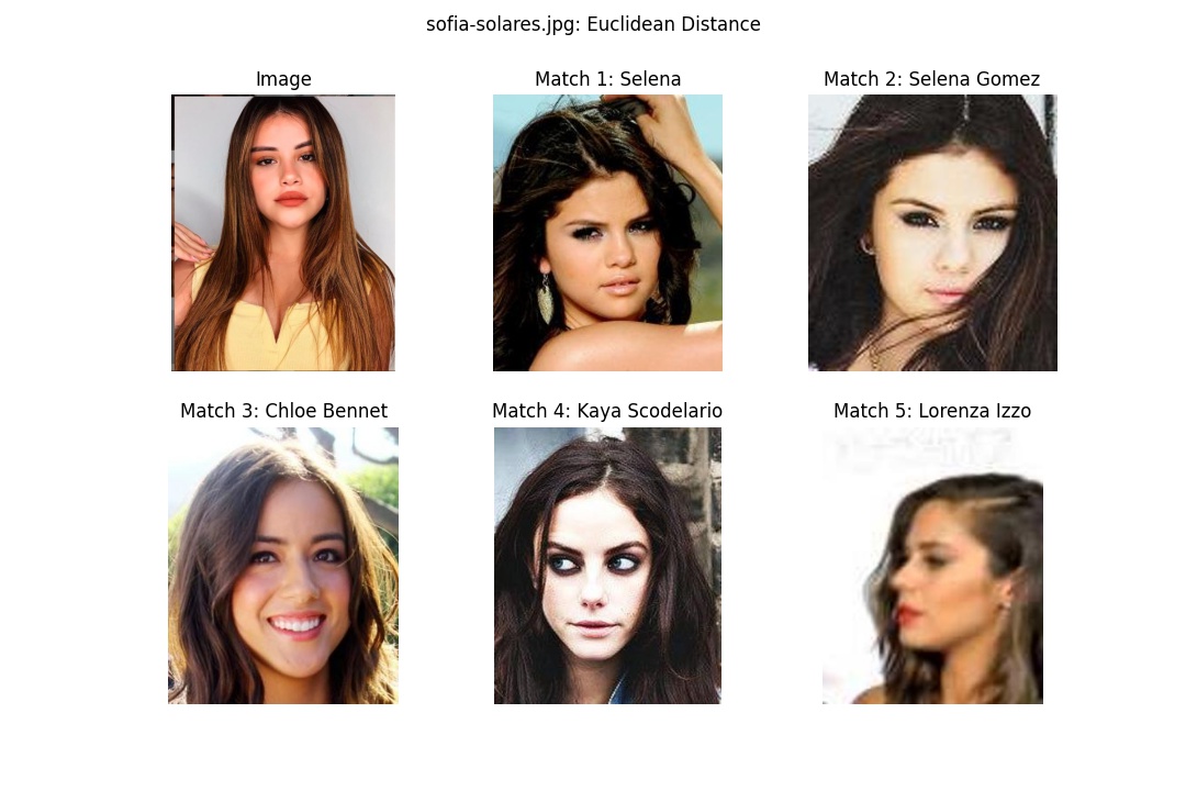
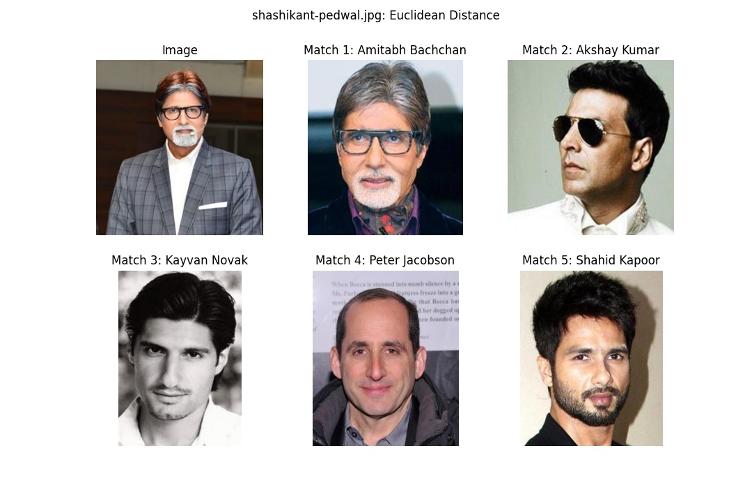
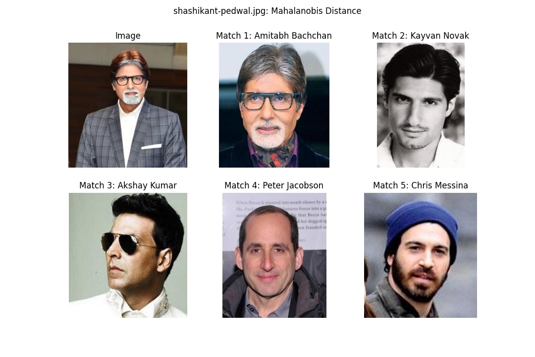
Because I was curious about not just the best identified match, I used my approach to find the best 5 matches for both of the two test images referenced in the Introduction section above. Without further ado, the results are presented below.

Image 1:

Euclidean distance

Mahalanobis distance

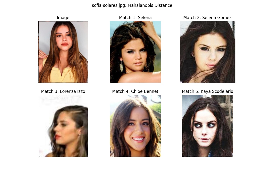
Image 2:

Euclidean distance

Mahalanobis distance

Discussion

Performance on test images

The discussion here will be brief, since the expected outcome of the project has been successfully demonstrated in the plots from the Results section above; the best match identified for each test image provided matches expectation. What I would like to highlight is the fact that the two approaches lead to similar results for the top, i.e. best, matches. In fact, based on similarity of results achieved for both methods, and the fact that the Euclidean distance approach was much easier to implement, I would focus further efforts with this particular method towards using the Euclidean distance for means of evaluating similarity.

One thing of note is that Matches 1 and 2 for Image 1 claim to represent two different celebrities, Selena and Selena Gomez, however the images representing Selena are, in fact, pictures of Selena Gomez. Since I didn’t have to train the model, this inconsistency in labeling isn’t a big deal, but if I were to refine the model by retraining on the celeb_mini dataset provided, I would merge the two separate folders into one. Moreover, I’d do a deeper dive into the dataset itself to make sure there were no other inconsistencies present.

Performance on other images

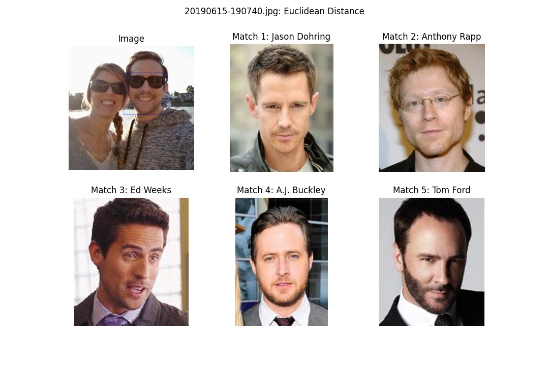
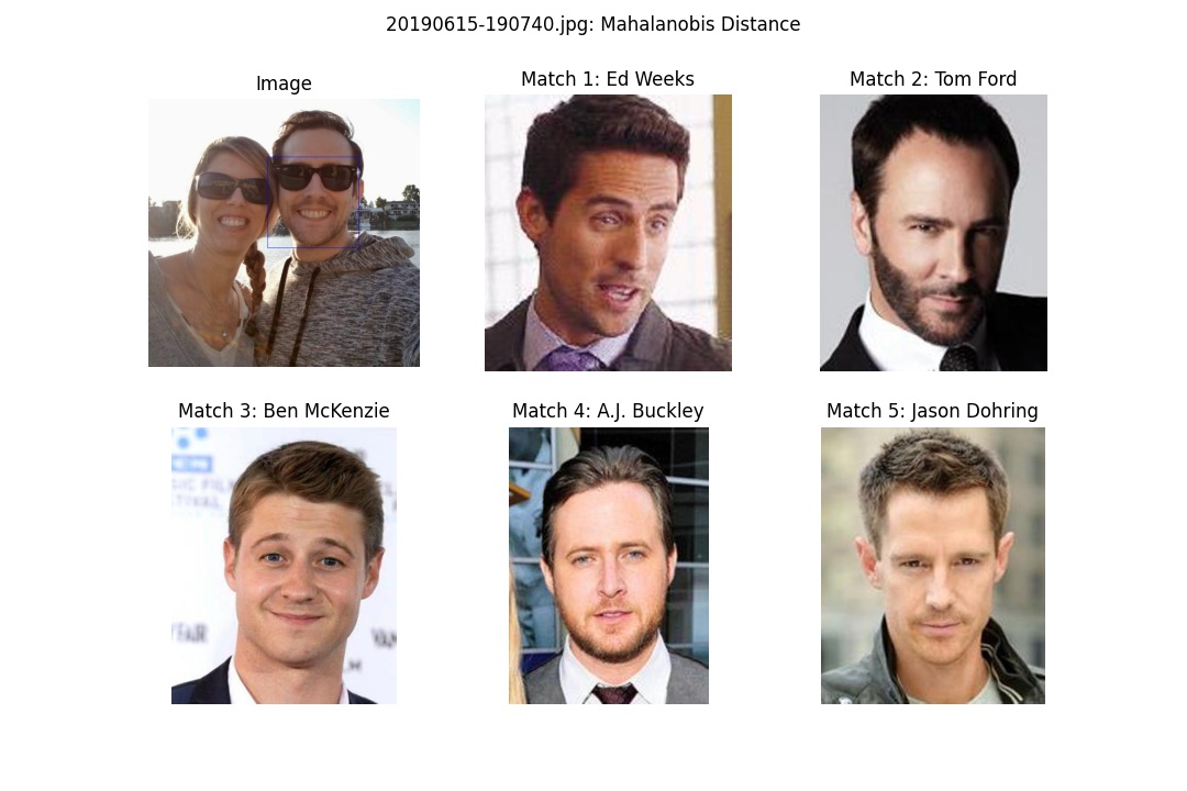
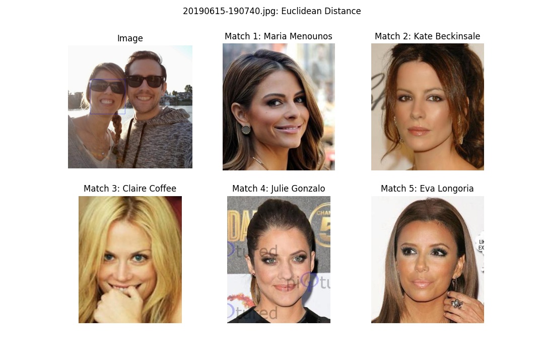
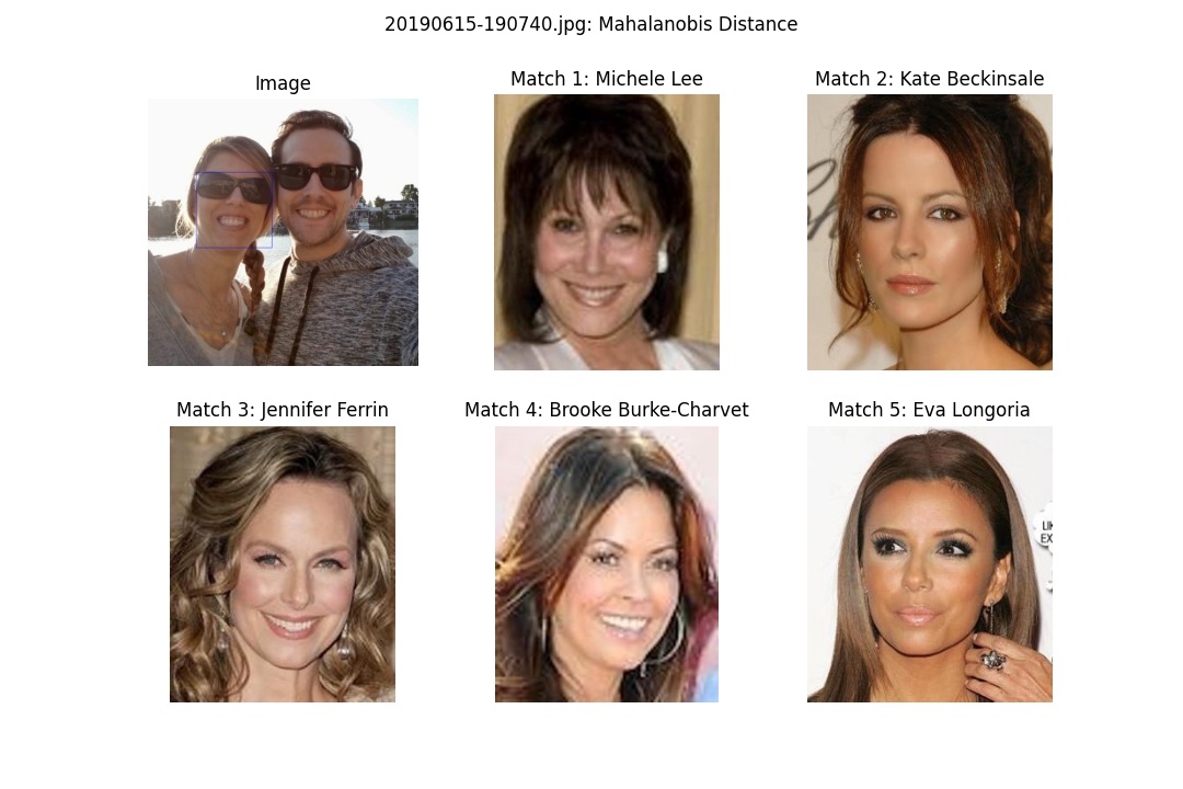
I was curious about what the approach would say about who the celebrity doppelgangers are for my wife and I and, as a follow-up, find out whether or not such predictions be common across different images (with different lighting, background, glasses/no-glasses, etc…). The results are shown below.

Image 3: My wife and I at a restaurant

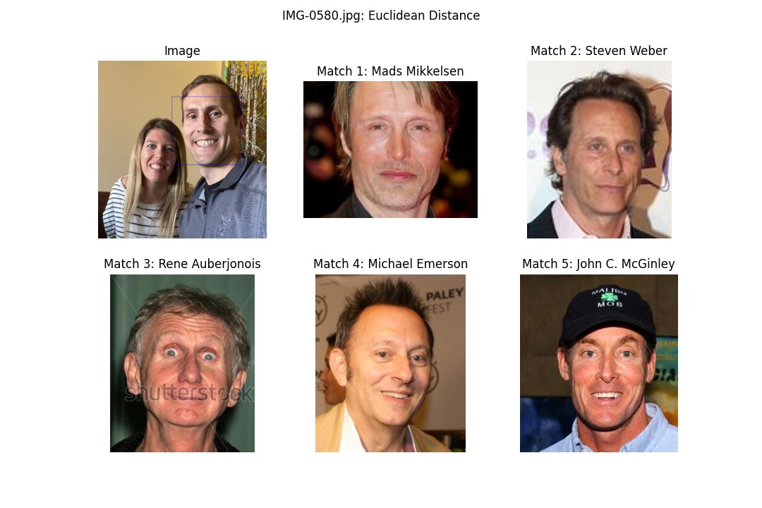
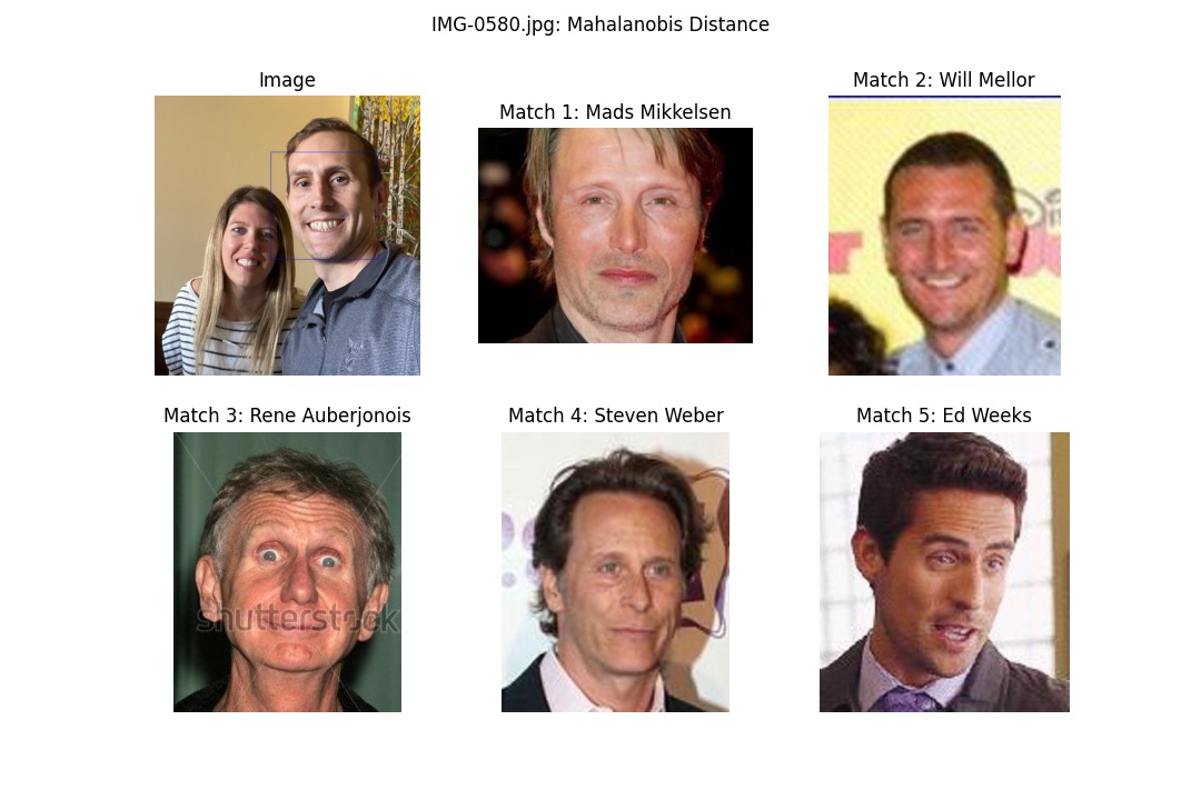
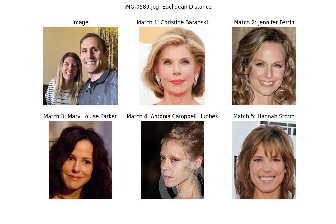
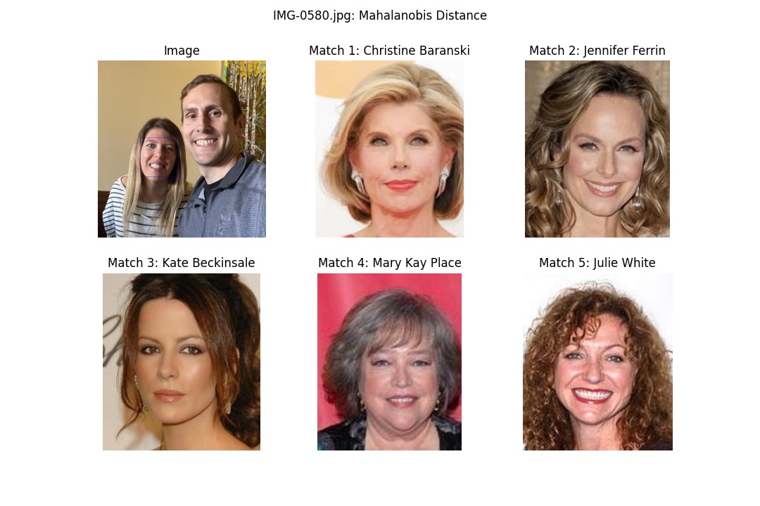
Note: to poke at the issue of data labeling yet again: the image shown for Match 4 is, in fact, an image of Kathy Bates, not Mary Kay Place.

Image 4: My wife and I near a lake at dusk

Final Remarks

Although there are some common matches between the two images for both my wife and myself, the top matches are different. Therefore it is expected that this approach would need considerable work to generalize to new images. To increase generalizability of the approach, I would try out the following approaches:

• Gather additional data. This is always the best approach if data is not difficult to gather (in this case, it wouldn’t be)
• Scrub the data and clean labels. In my limited investigations with the data, I found a few bogus examples (in terms of incorrect labeling), as well as some blurry, low-quality images.
• Retrain the model. This will definitely improve inter-class separation (w.r.t the metric loss function) among the classes present in the input dataset

I had a lot of fun working this project. After finishing, I have come to really appreciate the dlib C++ API; it provides so much functionality in one project: linear algebra, machine learning, multithreading, optimization, … the list goes on-and-on. I am really looking forward to working more with this library in future projects.

I know that I’ve only been able to highlight portions of the project above, but I’m happy to discuss the other aspects of the project over email or whatever (see contact info at the bottom of here).

I hope that you got something out of this post. Thanks for reading!