Implementation of different fixed-wing flight controllers
I have been working through the Small Unmanned Aircraft book by Beard and McLain this year and I want to write about some of the interesting concepts I have been exploring, some of which are covered in the book and some of which are not. The book does an excellent job of presenting the basics of small fixed-wing aircraft, including
- Vehicle modeling
- Flight dynamics
- Controller design
There is a draft update to the first edition of the book in the works that further develops additional concepts but I have found that some of the updated sections, particularly those concerning flight controls, have insufficient information to implement functional controllers. This post is my attempt to provide sufficient information to implement and test the LQR and nonlinear total energy control system (TECS) controllers described here and here, respectively.
Before reading through this post, it would help to review the first six chapters of the book or the corresponding lecture slides. In this post, I assume the reader is familiar with the following material from the book:
- fixed-wing vehicle model (Chapters 1-4)
- reduced linear models for lateral and longitudinal dynamics (Chapter 5)
- the main control objectives for a fixed-wing flight controller; namely, achieving desired
- course angle
- altitude, and
- airspeed
This post is broken up into three sections:
- Implementing successive loop closure
- Linear Quadratic Regulator (LQR) control
- Nonlinear TECS control
In the first section, I will present information that I found useful while implementing the controller described in the book. The second and third sections will present more details for the other approaches, including
- Background; i.e., the why
- Derivation; i.e., the what
- Implementation; i.e., the how
To ensure a fair comparison between the controllers, a common reference flight path that introduces step responses in all three control objectives, sometimes concurrently, is chosen. For each controller test scenario, the true vehicle state is used for feedback.
Implementing successive loop closure
This controller is described in Chapter 6 of the book. Read the book or the corresponding lecture slides for the derivation and relevant details. This controller’s design assumes that the dynamics between course, altitude, and airspeed are decoupled, which allows the three control objectives to be achieved with two independent controllers: one for lateral control (course) and one for longitudinal control (altitude and airspeed). Both controllers use PID - proportional, integral, derivative - to drive errors between the objective (reference) and system state to zero using state feedback.
The lateral controller consists of two main control loops, a higher-rate inner loop for roll control (implemented as a PD controller) and a lower-rate outer loop for course angle control (implemented as a PI controller). Less critical, but still important, is a low-pass filter to hold the sideslip angle at zero; i.e., counteract high-frequency disturbances to yaw/heading angle.
The longitudinal controller consists of two (outer) control loops. The first loop is for altitude control, which is achieved with an inner, high-rate loop for pitch angle (a PD controller) and a lower-rate outer loop for altitude control (a PI controller). The second control loop is for airspeed and is implemented as a PI controller.
The main idea with successive loop closure is to design inner loops so that they can be reasonably approximated by a DC gain in the next loop to close. Each loop is modeled as a second-order linear system with control damping and bandwidth as design parameters. One drawback of this approach is when there are multiple loops to close whereby modeling errors in innermost loops will greatly constrain stability margins and control bandwidth for outer loops. Despite this drawback, this controller is quite useful when for fixed-wing flight control.
The guidance for implementing and tuning this controller is summarized as follows:
- Integrals add delay and instability to control loops, so avoid them in high-rate roll and pitch loops
- Integrals are appropriate for correcting steady-state errors in low-rate outer loops on course, altitude, and airspeed
- Starting from the innermost control loop in each channel and working outward, choose the next loop’s bandwidth to be a multiple (>5) of the previous loop’s bandwidth.
Following the guidance, I was able to implement and test the successive loop closure controller.
The controller works well with only a moderate amount of tuning. I found that a bandwidth multiplier factor greater than 10, substantially greater for the altitude outer loop, worked well to handle step responses without ringing or instability.
Here are some of the salient points I discovered while tuning this controller:
- Selecting damping ratios greater than 1 for all loops, except roll, helped to avoid overshoot and ringing in observed system response to step input changes.
- A very responsive (i.e., high bandwidth) control loop is required for the innermost longitudinal control loop (on pitch angle from elevator command) to counteract the pull of gravity on the vehicle.
- Relative to the book’s recommendation of bandwidth multiplier of 5-10 between inner and outer loops, a significantly larger multiplier (=50) was selected for the pitch angle to altitude outer loop controller. This large multiplier was selected to eliminate ringing in altitude.
Pros and cons
Pros
- Simple design. The control problem is decomposed into smaller, manageable decoupled objectives.
- Few control knobs to tune. This makes optimal gain selection using coordinate-ascent or similar approach simpler.
- Control margins (gain and phase) are quantifiable using methods from linear systems analysis (i.e., using Bode or Nyquist plots).
Cons
- The actual system response to step input changes shows that the dynamics are not decoupled, as assumed. Step changes in altitude (controlled by the longitudinal controller) are shown to affect system response in course angle (controlled by the lateral controller).
- The system is slow to drive out errors because of the low bandwidth on outer control loops.
LQR control
Background
The goal of LQR is to design a controller for a linear system like the one above that minimizes an objective function, \(J\), of two inputs:
- \(\mathbf{x}\) is system error
- \(\mathbf{u}\) is control effort
LQR is an example of an optimal control law with two important constraints: both the objective function and the feedback take particular forms. The objective function is the integral:
\[J = \int_0^\infty \Bigl ( \mathbf{x}^T Q \mathbf{x} + \mathbf{u}^T R \mathbf{u} \Bigr ) dt\]where the matrices \(Q\) and \(R\) are design parameters that provide the designer flexibility in weighting system errors relative to control effort. The second constraint is that the feedback is linearly proportional to the system error; i.e., \(\mathbf{u} = -K \mathbf{x}\).
After selecting \(Q\) and \(R\), the gain \(K\) is computed such that the resulting feedback, \(\mathbf{u}\), minimizes the objective function defined for the system.
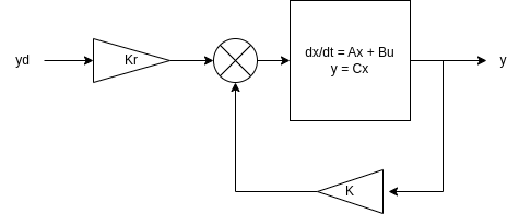
The feedback is only one part of the controller design though. There is a reference command, \(\mathbf{y}_d\) that we want the system to continuously follow. This input could be a step change in control objective or a trajectory. The reference could be tracked with feedback alone, however the addition of a feedforward term, \(K_r \mathbf{y}_d\), improves tracking performance when properly designed.
Derivation
Modeling the system
As in the successive loop closure control scheme described in the previous section, the vehicle controller is separated into two decoupled controllers for lateral and longitudinal dynamics. Each controller is designed around a common, fixed trim point; where the vehicle is in force- and moment-free equilibrium.
Finding a trim point
The book describes an optimization technique for finding the desired trim flight condition in Chapter 5. The inputs to the optimization are the following three quantities:
- The desired airspeed, \(V_a^*\)
- The desired flight path angle, \(\gamma^*\)
- The desired orbit radius, \(R^*\)
If the desired flight condition is level flight along a straight-line path, which is assumed for the LQR controller design, then \(\gamma^*=0\) and \(R^*=\infty\).
Linearization
The full system dynamics, as described in Chapter 3, are nonlinear. The LQR controller can only be applied to such systems after linearizing about a trim point. The controller that is designed will generate the control input to apply as a correction to the trim control input. For example, if the trim flight condition has throttle command, \(\delta_t^*\), and the LQR controller for the linearized system generates a throttle correction, \(u_{\delta_t}\), the total system throttle command would be \(\delta_t^* + u_{\delta_t}\).
Recall, both the lateral and longitudinal dynamics will take the form:
\[\begin{aligned} \dot{\mathbf{x}} &= A \mathbf{x} + B \mathbf{u} \\ \mathbf{y} &= C \mathbf{x} \end{aligned}\]The linearized dynamics for both the lateral and longitudinal systems are described in Chapter 5 of the book.
The feedback control input is: \(\mathbf{u}_{fb} = -K \mathbf{x}\). The feedforward control input is a linear combination of reference commands: \(\mathbf{u}_{ff} = K_r \mathbf{y}_d\). The total control input is the sum of these two terms:
\[\mathbf{u} = K_r \mathbf{y}_d - K \mathbf{x}\]The resulting controlled system dynamics are:
\[\begin{aligned} \dot{\mathbf{x}} &= (A - BK) \mathbf{x} + B K_r \mathbf{y}_d \\ \mathbf{y} &= C \mathbf{x} \end{aligned}\]Selecting the feedforward gain, \(K_r\)
The gain \(K_r\) is selected so that the steady-state output, \(\mathbf{y}_e\), equals the desired reference input, \(\mathbf{y}_d\). “Steady-state” means that the system is in equilibrium; i.e., \(\dot{\mathbf{x}} = \mathbf{0}\). It follows that:
\[\begin{aligned} \mathbf{0} &= (A - BK) \mathbf{x}_e + B K_r \mathbf{y}_d \\ \mathbf{y}_e &= C \mathbf{x}_e = \mathbf{y}_d \\ \mathbf{x}_e &= -(A - BK)^{-1} B K_r \mathbf{y}_d \end{aligned}\]These conditions lead to the following equality:
\[\begin{aligned} \mathbf{y}_d &= C \mathbf{x}_e = -C (A - BK)^{-1} B K_r \mathbf{y}_d \end{aligned}\]which implies that:
\[\begin{aligned} I &= -C (A - BK)^{-1} B K_r \\ \implies K_r &= -\bigl ( C (A - BK)^{-1} B \bigr )^{-1} \end{aligned}\]Feedback with integral action added
There will be modeling errors due to linearization and disturbances. A standard approach for dealing with such errors is to add an integral term by augmenting the state vector, \(\mathbf{x}\), with the vector \(\mathbf{z}\):
\[\begin{aligned} \mathbf{z}(t) &= \int_0^t (\mathbf{y}_d - C \mathbf{x}) dt \\ \dot{\mathbf{z}} &= \mathbf{y}_d -C \mathbf{x} \end{aligned}\]The resulting augmented system dynamics are:
\[\begin{aligned} \begin{bmatrix} \dot{\mathbf{x}} \\ \dot{\mathbf{z}} \end{bmatrix} &= \begin{bmatrix} A & \mathbf{0} \\ -C & \mathbf{0} \end{bmatrix} \begin{bmatrix} \mathbf{x} \\ \mathbf{z} \end{bmatrix} + \begin{bmatrix} B \\ \mathbf{0} \end{bmatrix} \mathbf{u} + \begin{bmatrix} \mathbf{0} \\ 1 \end{bmatrix} \mathbf{y}_d \\ \mathbf{y} &= \begin{bmatrix} C & \mathbf{0} \end{bmatrix} \begin{bmatrix} \mathbf{x} \\ \mathbf{z} \end{bmatrix} \end{aligned}\]Applying the LQR design process (see Chapter 9 of Friedland’s Control System Design book for details) to these augmented dynamics leads to the optimal linear feedback law:
\[\begin{aligned} \mathbf{u}_{fb} &= K_+ \mathbf{x}_+\\ &\triangleq - \begin{bmatrix} K & K_i \end{bmatrix} \begin{bmatrix} \mathbf{x} \\ \mathbf{z} \end{bmatrix} \end{aligned}\]The reason for breaking the augmented gain, \(K_+\) into two components, \(K\) and \(K_i\), is so that integrator windup can be mitigated. The consequence of integrator windup is that large integrated errors can force control inputs to saturate over time. Saturated control can drive the system unstable if applied for any appreciably long period of time.
Integrator anti-windup for scalar integral terms is described in Chapter 6 of the book. One of the proposed schemes for addressing windup can be modified to apply to the multivariate case. Let \(\Delta \mathbf{z}\) be the correction to apply to the integral term, \(\mathbf{z}\), so that the control input \(\mathbf{u}\) is no greater than its saturated value. In the equations that follow, the superscript \(.^-\) means the value before the correction \(\mathbf{z}\) has been applied. The correction is computed by solving the linear system:
\[\begin{aligned} K_i \Delta \mathbf{z} = \mathbf{u}^- - \mathbf{u}. \end{aligned}\]An important note here: the control vectors, \(\mathbf{u}^-\) and \(\mathbf{u}\) are representative of the sum of the trim control, the feedforward term, and the feedback term; i.e., the saturation is to be applied to the full control input, not just the feedforward and feedback terms derived in this section.
After computing the correction \(\Delta \mathbf{z}\), the stored value for the integral term \(\mathbf{z}\) is updated as \(\mathbf{z} = \mathbf{z}^- + \Delta \mathbf{z}\). From the form of the linear equation to solve, it is clear that, when the control vector has not saturated, the correction \(\Delta \mathbf{z}\) will be zero.
Following on the discussion from earlier in this section: if the augmented system dynamics are Hurwitz, then there is a theoretical guarantee that the system will reach \(\mathbf{y}_d\) in steady-state; i.e., as \(t \to \infty\) without feedforward. The inclusion of the feedforward term, \(K_r \mathbf{y}\), is therefore still not necessary to achieve the control objective \(\mathbf{y}_d\).
Implementation
The implementation of this controller is straightforward when following the material from Chapter 9 of Friedland’s book. The main consideration for controller performance is selection of the design parameters, \(Q\) and \(R\). Bryson and Ho provide the following guidance:
- Set the off-diagonal terms of both \(Q\) and \(R\) to \(0\).
- Set the diagonal terms of \(Q\) to the recriprocal of the expected squared error of the state.
- Set the diagonal terms of \(R\) to the reciprocal of the squared maximum control input.
Choosing the expected maximum errors for the elements of \(\mathbf{x}\) is straightforward, since the maximum expected step responses can be quantified. For the integral terms, the maximum expected error assumes linear decay of the error integrand over a desired decay time.
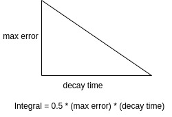
The maximum error chosen for the integral error is the same as for the corresponding element of \(\mathbf{x}\). The desired decay time is an additional design parameter. Choosing a shorter decay time means the controller will prioritize (relatively speaking) keeping the integrated error small.
Bryson’s rule is great as a general rule of thumb, but is not generally robust to unmodeled effects like disturbances or errors with the model. In this case, with the inclusion of moderate wind, the parameters selected using the rule provide good performance. In fact, the performance looks better than that of the successive loop closure approach with regards to the following:
- The output rings less in response to step input changes.
- Errors converge to 0 faster.
- There is less coupling between the different channels in response to step input changes.
Pros and cons
Pros
- The approach is mathematically rigorous; under certain assumptions, there is provable optimality of the control input computed.
- The coupling between states is accounted for directly in the model; at least to a first-order approximation.
- The controller is easy to implement, requiring only standard techniques from linear algebra.
Cons
- The controller is more complex than successive loop closure.
- The controller requires that the system be linearized about a trim point. In general, the further the state gets from the trim point, the less stable the system becomes.
- The selection of the design parameters, \(Q\) and \(R\), is non-trivial. Errors with the model, including disturbances, can be difficult to account for.
- There are no stability margin or robustness guarantees like there are when using frequency domain methods for linear systems.
Nonlinear TECS control
Background
The LQR longitudinal controller is one way of dealing with the dynamic coupling between airspeed and pitch angle. As shown in the previous section, the approach works well for the test case considered, where the vehicle remains acceptably close to the trim point throughout operation. The linearity of LQR is an issue for large deviations from the trim point; e.g., when the vehicle is initially ascending to a cruising altitude.
Total Energy Control System (TECS) is a control methodology that recognizes that commanding airspeed, \(V_a\), and (airmass adjusted) flight path angle, \(\gamma_a\), can be used to drive the total energy of the aircraft to a desired state. As opposed to the other controllers discussed, where the primary control objective is to drive system errors to zero, the objective of TECS-based controllers is to drive the system’s kinetic and potential energies to desired values. Kinetic energy is proportional to airspeed (squared) and potential energy is proportional to elevation. Airspeed, \(V_a\), is adjusted most directly through commanding throttle, and elevation is affected most directly by commanding flight path angle, \(\gamma_a\).
There are several approaches to implement a TECS-based controller. I will present a Lyapunov-based controller. This approach requires no trim point, so concerns about linearization present in LQR are not an issue.
Derivation
A more detailed derivation of the nonlinear TECS controller can be found Section IV of this paper. I will only discuss an outline of the approach, including whatever key assumptions are made along the way.
Recall the equations of kinetic and potential energies, \(E_K\) and \(E_P\), respectively:
\[\begin{aligned} E_K &= \frac{1}{2} m V_g^2 \\ E_P &= m g h \\ \end{aligned}\]where \(m, g, V_g\) and \(h\) are vehicle mass, gravitational acceleration at sea-level, ground speed, and altitude, respectively. The total energy, \(E_T\), is the sum of these two terms, whereas the energy difference, \(E_D\), is the difference, \(E_P - E_K\). If wind is assumed to be negligible, \(V_a = V_g\). This assumption is important: since the vehicle only commands and measures airspeed directly. The airspeed and altitude commands, \(V_a^d\) and \(h^d\), correspond directly to the desired energy of the system:
\[\begin{aligned} E_K^d &= \frac{1}{2} m \bigl( V_a^d \bigr )^2 \\ E_P^d &= m g h^d \\ E_T^d &\triangleq E_P^d + E_K^d \\ E_D^d &\triangleq E_P^d - E_K^d \end{aligned}\]The control objective is to drive the kinetic and potential energies to the desired values. A Lyapunov function in terms of the total energy and energy difference errors is chosen:
\[\begin{aligned} \tilde{E}_T &\triangleq E_T^d - E_T \\ \tilde{E}_D &\triangleq E_D^d - E_D \\ V &= \frac{1}{2} k_T \tilde{E}_T^2 + \frac{1}{2} k_D \tilde{E}_D^2. \end{aligned}\]Since \(V(t)\) must be positive semi-definite, i.e., \(V(t) \ge 0 \ \forall t\), the gains \(k_T\) and \(k_D\) must both be greater than or equal to 0. If a control input can be found such that \(\dot V < 0 \ \forall t\), then it is true that the control input drives the system energies to the desired values.
To find a control law that proves \(\dot V\) is strictly negative, \(V\) must be first written out in terms of the state variables \(V_a\) and \(h\) and differentiated. The result contains state derivatives for which a dynamics model must be assumed. A suitable and simple model is to assume that:
- The propeller thrust, \(T\), acts purely in the opposite direction as the aerodynamic drag, \(D\), and
- The climb rate of the aircraft is proportional to the airspeed and the airmass referenced flight path angle, \(\gamma_a\), which is the difference of the pitch angle, \(\theta\), and the angle-of-attack, \(\alpha\)
or, in mathematical notation:
\[\begin{aligned} \dot V_a &= \frac{T-D}{m} - g \sin \theta \\ \dot h &= V_a \sin \gamma_a \end{aligned}\]Differentiating \(V\) and applying the model described above leads to the following control law:
\[\begin{aligned} T &= D + \frac{\dot E_T^d}{V_a} + k_T \frac{\tilde{E}_T}{V_a} \\ \theta &= \alpha + \sin^{-1} \biggl [ \frac{\dot h^d}{V_a} + \frac{1}{2mgV_a} \bigl( k_T \tilde{E}_T + k_D \tilde{E}_D \bigr ) \biggr ] \end{aligned}\]All that remains is to choose a model for the desired airspeed and climb rates that are used in the thrust command, \(T\). The simplest such model is first-order and proportional to the error between the desired and current states:
\[\begin{aligned} \dot V_a^d &= k_{V_a} (V_a^d - V_a) \\ \dot h^d &= k_h (h^d -h) \end{aligned}\]Implementation
The TECS approach applies only to the longitudinal channel so a lateral controller must be implemented separately. I chose to take the successive loop closure PID-based controller, but the LQR controller could have been chosen. Notice that the control law from the previous section defines commanded thrust and flight path angle. The expected control inputs are throttle and elevator, so a conversion between derived and actual controls is needed.
Thrust is a nonlinear function of throttle and airspeed. I used this relationship to build a lookup table from thrust and airspeed to commanded throttle. The alternative is to do a computationally expensive root finding operation each control iteration, which works fine for simulation but would likely be too slow in an actual flight controller to meet real-time requirements. The elevator command comes from a PD controller on pitch error; the same as in the successive loop closure case but with different gains.
The paper shows that \(k_D\) should be greater than or equal to \(k_T\) and provides reference values for them. In practice, I found setting these terms (about 2 times) larger made the controller more responsive without negatively affecting performance. I found that the choice of gains \(k_{V_a}\) and \(k_h\) had significant impact on the overall responsiveness of the controller: setting the gains higher (>1) led to fast response but with a lot of ringing, whereas gains near 1 provided a good balance between response and settling times.
While implementing this controller, I observed steady-state errors on airspeed and/or altitude. These errors are likely caused by the ground speed not being equal to the airspeed when wind is present. To remove these steady state errors I added a simple PI controller on each channel with small gains, which provides a slight correction to remove any steady-state errors. I didn’t spend a significant amount of time in tuning these corrective controllers; choosing small gains between 0.1 and 0.3 seemed to work well enough without additional consideration.
Pros and cons
Pros
- The controller is mathematically rigorous.
- The coupling between airspeed and altitude is accounted for.
- System errors are driven down much faster by this controller.
- No linearization is required.
- There are fewer control parameters than any of the other controllers considered.
Cons
- The controller only applies to the longitudinal channel.
- The assumption that ground speed and airspeed are the same leads to steady-state errors that must be handled independently.
- The controller is the most complex of the controllers considered.
Summary
Three flight control schemes for a simulated fixed-wing aircraft were presented and applied to a common test case with step disturbances on feedforward reference commands and moderate wind effects. The successive loop closure controller was the simplest and easiest to implement, however it was difficult to tune and did not properly account for coupling between the different state terms. The LQR controller performed well, but it required finding a trim point and linearizing about it. To account for large deviations from the trim point; e.g., when a large step response in input command is requested, the control design parameter \(Q\) must be selected to lower the control bandwidth, which will affect how responsive the controller is. The TECS-based controller performed the best of all controllers, but it only works on the longitudinal channel and is very complex.
Based on these observations, I think that the best flight controller that can be built from the options presented combines the lateral channel of the LQR controller with the TECS longitudinal controller; see GitHub for the implementation.
Thanks for reading!