State estimation for fixed-wing UAV

As mentioned in a previous post, I have been working through the Small Unmanned Aircraft book by Beard and McLain. In the aforementioned post, I presented implementations for fixed-wing UAV flight controllers. For the state feedback, the true states from the simulation are used. True state information is not available in actual UAV applications so estimates must be made using onboard sensor measurements; e.g., from GPS, altimeters, airspeed sensors, magnetometers, and accelerometers. In this post

In working through the estimation techniques of Chapter 8, I applied additional techniques to improve the state estimate. After discussing these techniques, I will present my implementation of the estimator.

Before reading this post, I suggest reviewing chapters 7 and 8 of the book or the corresponding lecture slides. You should also understand the wind triangle relationships from Chapter 2 (pg. 22).

Additional techniques

Add magnetometer measurements

Magnetometer models for measuring heading are presented in Chapter 7 of the book and lecture slides. I found the derivation of these models to be unclear and incomplete so I decided to work out the details of the model for myself.

Let \(B\) be the magnetic field strength at the vehicle’s location. The vector for magnetic north with origin at the vehicle center, \(\mathbf{m}^m\), can be expressed as \(\mathbf{m}^m = [B, 0, 0]^T\). The magnetic inclination, \(\iota\), and declination, \(\delta\), can be used to find the relationship between magnetic and true (geographic) north:

\[\begin{aligned} \mathbf{m}^i &\triangleq R(0, -\iota, \delta) \mathbf{m}^m \\ &= \begin{bmatrix} \cos \delta & -\sin \delta & 0 \\ \sin \delta & \cos \delta & 0 \\ 0 & 0 & 1 \end{bmatrix} \ \begin{bmatrix} \cos \iota & 0 & -\sin \iota \\ 0 & 1 & 0 \\ \sin \iota & 0 & \cos \iota \end{bmatrix} \mathbf{m}^m \\ &= B \begin{bmatrix} \cos \delta \cos \iota \\ \sin \delta \cos \iota \\ \sin \iota \end{bmatrix} \end{aligned}\]

where, \(\mathbf{m}^i\), is magnetic north expressed in a local NED coordinate frame. Declination, inclination, and field strength are functions of latitude and longitude on the Earth’s surface; see here for more information on these quantities. Practically speaking, values for these quantities can be found using a table lookup. For this post, I assume the values from the book: \(\delta = 12.5^{\circ}\), \(\iota = 66^{\circ}\) (near Provo, UT).

The magnetometer is composed of three orthogonal sensors designed to measure magnetic field strength along each body axis: \(b_x\), \(b_y\), and \(b_z\). Let \(\mathbf{m}^b \triangleq [b_x, b_y, b_z]^T\) be the measurement vector. It follows that:

\[\begin{aligned} R_b^i \mathbf{m}^b &= \mathbf{m}^i \\ R_{v_2}^{v_1} (\theta) R_{b}^{v_1}(\phi) \mathbf{m}^b &= R_i^{v_1} (\psi) \mathbf{m}^i \end{aligned}\]

where \(\theta\) and \(\phi\) are the estimated pitch and roll angles from the attitude filter described in the book. The intermediate coordinate frames, \(v_1\) and \(v_2\), are as defined in the book. To solve for \(\psi\), look at the three equalities derived from the expression above:

\[\begin{aligned} B \begin{bmatrix} \cos \psi \cos \iota \cos \delta + \sin \psi \cos \iota \sin \delta \\ -\sin \psi \cos \iota \cos \delta + \cos \psi \cos \iota \sin \delta \\ \sin \iota \\ \end{bmatrix} &= \begin{bmatrix} b_x \cos \theta + b_y \sin \phi \sin \theta + b_z \cos \phi \sin \theta \\ b_y \cos \phi - b_z \sin \phi \\ -b_x \sin \theta + b_y \sin \phi \cos \theta + b_z \cos \phi \cos \theta \end{bmatrix} \end{aligned}\]

Note that when declination is negligible, as assumed in Peter Corke’s video, the expression for \(\psi\) is simply:

\[\psi = \tan^{-1} \frac{\cos \theta ( b_z \sin \phi - b_y \cos \phi)}{b_x + B \sin \iota \sin \theta}\]

To estimate \(\psi\) without assuming declination is zero, either the root of one of the first two elements of the vector equality must be evaluated, or the minimum of a convex error function involving both terms must be found. The second approach worked better for me in practice:

\[\begin{aligned} e_1(\psi) &\triangleq B (\cos \psi \cos \iota \cos \delta + \sin \psi \cos \iota \sin \delta) \\ &- b_x \cos \theta - b_y \sin \phi \sin \theta - b_z \cos \phi \sin \theta \\ e_2(\psi) &\triangleq B (-\sin \psi \cos \iota \cos \delta + \cos \psi \cos \iota \sin \delta) \\ &- b_y \cos \phi + b_z \sin \phi \\ \psi &= \arg \min \bigl ( e_1^2 + e_2^2 \bigr ) \end{aligned}\]

Add altitude and flight path angle to GPS model while removing heading angle

Incorporating the magnetometer measurement in the attitude estimation makes heading directly observable. This is an improvement over the GPS model wherein heading is inferred from a dynamics model. The value from the attitude estimator is used for heading in the GPS model.

The GPS model presented in the book is planar: no consideration of change along the \(z\)-axis is considered. Adding altitude, \(h\), and flight path angle, \(\gamma\), makes motion in the vertical plane observable. Except for the following updates, all quantities in the GPS measurement model remain the same:

\[\begin{aligned} V_g &= \sqrt{\bigl( V_a \cos \psi \cos \gamma_a + w_n \bigr)^2 + \bigl( V_a \sin \psi \cos \gamma_a + w_e \bigr)^2 + \bigl( -V_a \sin \gamma_a + w_d \bigr)^2} \\ &\triangleq \sqrt{V_n^2 + V_e^2 + V_d^2} \\ \chi &= \tan^{-1} \frac{V_a \sin \psi \cos \gamma_a + w_e}{V_a \cos \psi \cos \gamma_a + w_n} \\ &\triangleq \tan^{-1}\frac{V_e}{V_d} \\ \gamma &= \sin^{-1} \frac{-(-V_a \sin \gamma_a + w_d)}{V_g} \\ &\triangleq - \sin^{-1}\frac{V_d}{V_g} \end{aligned}\]

Level flight \((\gamma = 0)\) is no longer assumed, so the pseudo measurement model becomes:

\[\begin{aligned} y_{\text{wind},n} &= V_a \cos \psi + w_n - V_g \cos \chi \cos \gamma \\ &\triangleq V_n - V_n' \\ y_{\text{wind},e} &= V_a \sin \psi + w_e - V_g \sin \chi \cos \gamma \\ &\triangleq V_e - V_e' \\ y_{\text{wind},d} &= w_d + V_g \sin \gamma \\ &\triangleq V_d - V_d' \end{aligned}\]

It is assumed that \(\gamma_a \triangleq \theta - \alpha = 0\).

The GPS process model becomes:

\[\begin{aligned} \begin{bmatrix} \dot p_n \\ \dot p_e \\ \dot p_d \\ \dot V_g \\ \dot \chi \\ \dot \gamma \\ \dot w_n \\ \dot w_e \\ \dot w_d \end{bmatrix} = \begin{bmatrix} V_n' \\ V_e' \\ V_d' \\ \frac{V_n \dot V_n + V_e \dot V_e + V_d \dot V_d}{V_g} \\ \frac{\dot V_e V_n - \dot V_n V_e}{V_e^2 + V_n^2} \\ -\Bigl ( \frac{1}{\sqrt{V_n^2 + V_e^2}} \Bigr ) \frac{\dot V_d V_g - \dot V_g V_d}{V_g} \\ 0 \\ 0 \\ 0 \end{bmatrix} \end{aligned}\]

Note the difference in the expression for \(\dot \chi\); the book uses a coordinated turn model for the expression whereas my approach uses the derivative of the exact expression directly.

Quantify variances explicitly

Before reading through this section, I encourage you to review how variance propagates when there is a functional relationship with quantities whose variance is known.

Process

The book doesn’t specify how to set the \(Q\) matrices for the two EKFs presented. For the attitude EKF, the equations-of-motion for the model are exact (i.e., they match the true dynamics) so the process model only needs to account for errors in the inputs to the model: \(p, q,\) and \(r\). These parameters come from a low-pass filter applied to gyro measurements.

For the GPS EKF, the process model assumes zero acceleration, so any acceleration of the actual vehicle needs to be accounted for as noise in the model. Assuming that \(\sigma_{\text{accel}}\) is the standard deviation of the acceleration per channel, the process noise \(Q\) becomes:

\[Q = \text{diag} \begin{bmatrix} (\sigma_{\text{accel}} \Delta t)^2 \\ (\sigma_{\text{accel}} \Delta t)^2 \\ (\sigma_{\text{accel}} \Delta t)^2 \\ 3 \sigma_{\text{accel}}^2 \\ 2 \frac{\sigma_{\text{accel}}^2}{V_g} \\ 2 \frac{\sigma_{\text{accel}}^2}{V_g} \\ \sigma_{\text{wind}}^2 \\ \sigma_{\text{wind}}^2 \\ \sigma_{\text{wind}}^2 \end{bmatrix}\]

The wind velocity is assumed to be in steady state, so any change is modeled as noise (with standard deviation \(\sigma_{\text{wind}}\)).

Measurements

The low-pass filter and GPS measurement models presented provide a means of calculating expected (mean) values for directly observable states, but no such method is provided for expressing the uncertainty (variance) of those estimates.

Recall the recursive low-pass filter presented in Chapter 8:

\[y_{n+1} = \alpha y_n + (1 - \alpha) u_n\]

where \(y_n\) and \(u_n\) are the state estimate and measurement at time \(n\), respectively. Using induction, the contribution of every prior measurement to the current estimate is written as:

\[y_{n} = \alpha^n u_0 + (1-\alpha) \sum_{i=1}^n \alpha^{n-i} u_i\]

Assuming that the measurement variance, \(\sigma_{uu}\), is constant at each measurement step, the expression for the estimate variance, \(\sigma_{y_{n}y_{n}}\), is found inductively to be:

\[\begin{aligned} \sigma_{y_{n}y_{n}} &= \biggl [ \Bigl(\frac{\partial y_n}{\partial u_0} \Bigr )^2 + \dots + \Bigl(\frac{\partial y_n}{\partial u_{n-1}} \Bigr)^2 \biggr ] \sigma_{uu} \\ &= \Bigl [\alpha^{2n} + (1-\alpha)^2 \sum_{i=0}^{n-1} \alpha^{2i} \Bigr ] \sigma_{uu}. \end{aligned}\]

The sum in the expression above is a geometric series, so it follows that:

\[\begin{aligned} \sigma_{y_{n}y_{n}} &= \biggl [\alpha^{2n} + (1-\alpha)^2 \frac{1-\alpha^{2n}}{1-\alpha^2} \biggr ] \sigma_{uu} \end{aligned}\]

Using the same methodology, the recursive relationship for the GPS error is found to be:

\[\begin{aligned} \sigma_{\nu_{n}\nu_{n}} &= \Bigl ( \sum_{i=0}^n a^{n - i} \Bigr ) \sigma_{\eta_{\text{GPS}} \eta_{\text{GPS}}} \\ &= \frac{1 - a^{n+1}}{1-a} \sigma_{\eta_{\text{GPS}} \eta_{\text{GPS}}} \end{aligned}\]

where \(a \triangleq e^{-k_{\text{GPS}} T_s}\). Refer to Section 7.5 in the book for more details.

These expressions are derived using the univariate form of the propagation of uncertainty method. There is a multivariate form of this method:

\[\begin{aligned} \Sigma_{\mathbf{y}} &= J \Sigma_{\mathbf{x}} J^T \end{aligned}\]

where \(\mathbf{y} = \mathbf{f}(\mathbf{x})\) and \(J\) is the Jacobian of \(\mathbf{f}\) with respect to (wrt) \(\mathbf{x}\): \(\Bigl [ \frac{\partial f_i}{\partial x_j} \Bigr ]_{ij}\).

The uni- and multivariate forms of uncertainty propagation are used in my implementation to provide well-reasoned, quantifiably correct estimates of process and measurement noise in the Kalman filter equations.

Error in the accelerometer measurement model

The accelerometer measurement model assumes the vehicle is in equilibrium, so this needs to be accounted for in the measurement noise. To quantify the error, I generated the following chart showing the difference between the actual acceleration and the output of the measurement model:

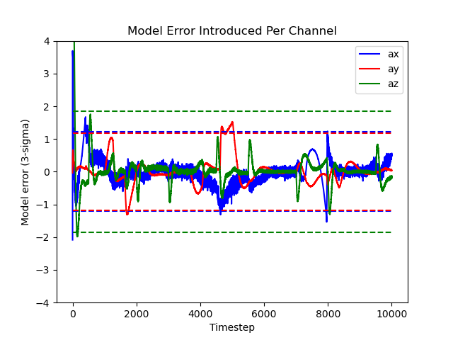
A conservative variance estimate based on these data is added to the accelerometer measurement noise to handle measurement updates for the model. The dashed lines represent the 3-\(\sigma\) bounds. The data is well-approximated by a zero mean Gaussian distribution.

Fuse independent estimates

Altitude is directly observable from two independent measurement sources: the GPS and the altimeter. The GPS measurement is incorporated into a position estimator (using a Kalman filter), whereas the altimeter measurements are fed into a low-pass filter. Both of these approaches, after using the uncertainty quantification method from the previous section, have well-defined mean and variance. These quantities can be fused to provide a better (i.e., smaller variance) estimate for altitude:

\[\begin{aligned} h &= h_{\text{alt}} + K \bigl (h_{\text{GPS}} - h_{\text{alt}} \bigr ) \\ \sigma_{hh} &= (1 - K) \sigma_{h_{\text{alt}} h_{\text{alt}}} \\ K &= \frac{\sigma_{h_{\text{alt}} h_{\text{alt}}}}{\sigma_{h_{\text{alt}} h_{\text{alt}}} + \sigma_{h_{\text{GPS}} h_{\text{GPS}}}} \end{aligned}\]

Note that the relationship above looks a lot like the Kalman filter update equations; the “prior” (\(h_{\text{alt}}\) in this context) and its variance (\(\sigma_{h_{\text{alt}} h_{\text{alt}}}\)) are combined with a “measurement” update (\(h_{\text{GPS}}\)) and its variance (\(\sigma_{h_{\text{GPS}} h_{\text{GPS}}}\)) optimally assuming that the prior and measurement models are Gaussian distributed about the true altitude.

Implementation

GitHub

My implementation uses the successive loop closure flight controller described here. You can see from the video above that the estimator works pretty well:

• Heading, pitch, roll, and course angle estimates are never more than a few degrees from the actual values
• Position errors are considerably less than 1m; most often times the errors are only a few centimeters.
• Velocity errors are very small
• Wind estimates converge quickly when the vehicle is not maneuvering. When the vehicle maneuvers, the estimator has difficulty rejecting the hypothesis that the wind is what’s causing the maneuver. This could be addressed by trying either (or both):
  • reducing \(\sigma_{\text{wind}}\), or
  • increasing \(\sigma_{\text{accel}}\).

The best words of advice/caution I can give to would-be implementors are:

• Start by getting the attitude estimator working properly. This estimator is less complex because it has fewer dimensions and there are no process model assumptions that need to be accounted for.
• Set a reasonable gating threshold for the GPS measurement updates. I couldn’t get the estimator to work properly when gating aggressively, but I think that a balance needs to be struck that still throws out outliers.
• Use Zarchan’s method to inflate the process noise covariance to aid the estimator in better balancing the incorporation of the prior into the posterior estimate.
• Lower the controller gains considerably (~30-50%) from the Chapter 6 implementation of flight controllers. Otherwise, your vehicle will have low amplitude, high frequency oscillations throughout flight; particularly so in the pitch channel.

Summary

I presented my additions to the observer model presented in the Small Unmanned Aircraft book, as well as a functional implementation. I learned a lot about how finnicky estimators can be and I hope this post helps the person who reads it avoid some of the pitfalls I encountered while working through this part of the book. At some point in the future (definitely not anytime soon), I would like to implement a complete state estimator that includes biases, wind angles \(\alpha\) and \(\beta\), and drag force. Having an estimate for drag will allow me to use the nonlinear TECS flight controller I wrote about last time.

Thanks for reading!