Smartcab Training
Reinforcement Learning
Abstract
This is a project that I completed as part of Udacity’s machine learning nanodegree. Given a basic Python simulator, I was able to use a Q-learning scheme to teach a smartcab to drive safely and efficiently towards a desired goal.
Getting Started
In this project, you will work towards constructing an optimized Q-Learning driving agent that will navigate a Smartcab through its environment towards a goal. Since the Smartcab is expected to drive passengers from one location to another, the driving agent will be evaluated on two very important metrics: Safety and Reliability. A driving agent that gets the Smartcab to its destination while running red lights or narrowly avoiding accidents would be considered unsafe. Similarly, a driving agent that frequently fails to reach the destination in time would be considered unreliable. Maximizing the driving agent’s safety and reliability would ensure that Smartcabs have a permanent place in the transportation industry.
Safety and Reliability are measured using a letter-grade system as follows:
| Grade | Safety | Reliability |
|---|---|---|
| A+ | Agent commits no traffic violations, and always chooses the correct action. | Agent reaches the destination in time for 100% of trips. |
| A | Agent commits few minor traffic violations, such as failing to move on a green light. | Agent reaches the destination on time for at least 90% of trips. |
| B | Agent commits frequent minor traffic violations, such as failing to move on a green light. | Agent reaches the destination on time for at least 80% of trips. |
| C | Agent commits at least one major traffic violation, such as driving through a red light. | Agent reaches the destination on time for at least 70% of trips. |
| D | Agent causes at least one minor accident, such as turning left on green with oncoming traffic. | Agent reaches the destination on time for at least 60% of trips. |
| F | Agent causes at least one major accident, such as driving through a red light with cross-traffic. | Agent fails to reach the destination on time for at least 60% of trips. |
To assist evaluating these important metrics, you will need to load visualization code that will be used later on in the project. Run the code cell below to import this code which is required for your analysis.
# Import the visualization code
import visuals as vs

# Pretty display for notebooks
%matplotlib inline
Understand the World
Before starting to work on implementing your driving agent, it’s necessary to first understand the world/environment which the Smartcab and driving agent work in. One of the major components to building a self-learning agent is understanding the characteristics about the agent, which includes how the agent operates. To begin, simply run the agent.py agent code exactly how it is – no need to make any additions whatsoever. Let the resulting simulation run for some time to see the various working components. Note that in the visual simulation, if enabled, the white vehicle is the Smartcab.
Question 1
In a few sentences, describe what you observe during the simulation when running the default agent.py agent code. Some things you could consider:
- Does the Smartcab move at all during the simulation?
- What kind of rewards is the driving agent receiving?
- How does the light changing color affect the rewards?
Hint: From the /smartcab/ top-level directory, run the command
'python smartcab/agent.py'
Answer:
The smartcab doesn’t move during any of the individual trials. At the inception of each trial, the initial position of the smartcab is updated to a new location. The smartcab receives rewards for reacting to lights. The rewards appear to fluctuate in value in response to nearby traffic; I observed a higher reward while the cab stayed stopped at a red light while a car travelled through the intersection perpendicularly to the smartcab. While the light is red, the smartcab receives a positive reward, while it receives a negative reward, or penalty, while the light is green.
Understand the Code
In addition to understanding the world, it is also necessary to understand the code itself that governs how the world, simulation, and so on operate. Attempting to create a driving agent would be difficult without having at least explored the “hidden” devices that make everything work. In the /smartcab/ top-level directory, there are two folders: /logs/ which will be used later and /smartcab/. Open the /smartcab/ folder and explore each Python file included, then answer the following question.
Question 2
- In the
agent.pyPython file, choose three flags that can be set and explain how they change the simulation. - In the
environment.pyPython file, what Environment class function is called when an agent performs an action? - In the
simulator.pyPython file, what is the difference between therender_text()function and therender()function? - In the
planner.pyPython file, will thenext_waypoint()function consider the North-South or East-West direction first?
Answer:
In agent.py, setting the flag learning true forces the agent to use Q-learning, otherwise random actions are chosen. The flag display set to false turns off the simulation GUI when PyGame is enabled. The flag n_test changes the number of trials that are run by the simulation.
In the file environment.py, the act class function is called when an agent performs an action.
In the file simulator.py, the render_text() function posts text data output from the simulation to the terminal window while the render() function is responsible for populating the GUI with sim data.
In the file planner.py, the next_waypoint() function considers the East-West direction first.
Implement a Basic Driving Agent
The first step to creating an optimized Q-Learning driving agent is getting the agent to actually take valid actions. In this case, a valid action is one of None, meaning take no action, 'Left' meaning turn left, 'Right' meaning turn right, or 'Forward' meaning go forward. For your first implementation, navigate to the 'choose_action()' agent function and make the driving agent randomly choose one of these actions. Note that you have access to several class variables that will help you write this functionality, such as 'self.learning' and 'self.valid_actions'. Once implemented, run the agent file and simulation briefly to confirm that your driving agent is taking a random action each time step.
Basic Agent Simulation Results
To obtain results from the initial simulation, you will need to adjust following flags:
-
'enforce_deadline'- Set this toTrueto force the driving agent to capture whether it reaches the destination in time. -
'update_delay'- Set this to a small value (such as0.01) to reduce the time between steps in each trial. -
'log_metrics'- Set this toTrueto log the simluation results as a.csvfile in/logs/. -
'n_test'- Set this to'10'to perform 10 testing trials.
Optionally, you may disable to the visual simulation, which might make the trials go faster, by setting the 'display' flag to False. Flags that have been set here should be returned to their default setting when debugging. It is important that you understand what each flag does and how it affects the simulation!
Once you have successfully completed the initial simulation, there should have been 20 training trials and 10 testing trials, run the code cell below to visualize the results. Note that log files are overwritten when identical simulations are run, so be careful with what log file is being loaded!
# Load the 'sim_no-learning' log file from the initial simulation results
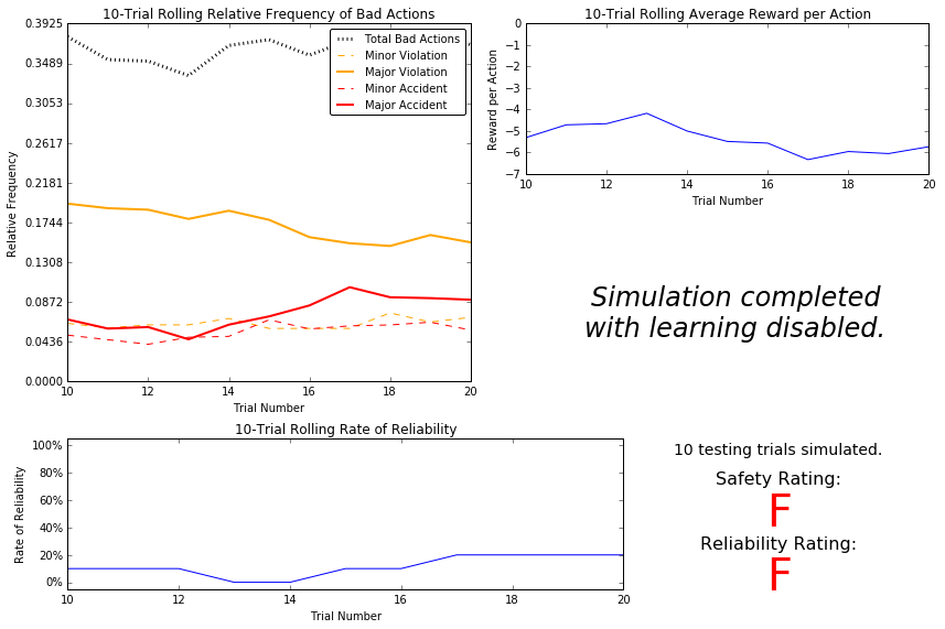
vs.plot_trials('sim_no-learning.csv')
Question 3
Using the visualization above that was produced from your initial simulation, provide an analysis and make several observations about the driving agent. Be sure that you are making at least one observation about each panel present in the visualization. Some things you could consider:
- How frequently is the driving agent making bad decisions? How many of those bad decisions cause accidents?
- Given that the agent is driving randomly, does the rate of reliability make sense?
- What kind of rewards is the agent receiving for its actions? Do the rewards suggest it has been penalized heavily?
- As the number of trials increases, does the outcome of results change significantly?
- Would this Smartcab be considered safe and/or reliable for its passengers? Why or why not?
Answer:
From the upper-left plot, it can be seen that the driving agent makes bad decisions about 40% of the time resulting in between a 4.8% and 8% incidence of major accidents and between 4% and 5% incidence of minor accidents. Doing some quick math, it appears that between 1-in-8 and 1-in-5 of these bad decisions result in major accidents and between 1-in-10 and 1-in-8 of these bad decisions result in minor accidents. Considering that the agent employs a random driving strategy, the reliability rate seems reasonable. I would expect perhaps one run in ten would be successful given the fact that, given enough time, a random walk will visit all points on a grid. The average reward that the agent receives for its actions is very negative relative to the policies for staying still at a green light. It seems that the agent is being heavily penalized, and the incidence of accidents, both major and minor, confirms that it is reasonable to expect a large penalty for the random policy employed. As the number of trials increases, none of the observed outputs vary significantly.
From the observed data, this smartcab would be considered neither safe nor reliable for passengers. A 40% incidence of bad actions would be terrifying to experience in a cab; although, in Mexico, this is perhaps close to the norm ![]() . The near 13% chance of either a major or minor accident occurring is far too unsafe for a commercial cab venture, and the random policy is clearly unreliable, as seen in the bottom right plot.
. The near 13% chance of either a major or minor accident occurring is far too unsafe for a commercial cab venture, and the random policy is clearly unreliable, as seen in the bottom right plot.
Inform the Driving Agent
The second step to creating an optimized Q-learning driving agent is defining a set of states that the agent can occupy in the environment. Depending on the input, sensory data, and additional variables available to the driving agent, a set of states can be defined for the agent so that it can eventually learn what action it should take when occupying a state. The condition of 'if state then action' for each state is called a policy, and is ultimately what the driving agent is expected to learn. Without defining states, the driving agent would never understand which action is most optimal – or even what environmental variables and conditions it cares about!
Identify States
Inspecting the 'build_state()' agent function shows that the driving agent is given the following data from the environment:
-
'waypoint', which is the direction the Smartcab should drive leading to the destination, relative to the Smartcab’s heading. -
'inputs', which is the sensor data from the Smartcab. It includes-
'light', the color of the light. -
'left', the intended direction of travel for a vehicle to the Smartcab’s left. ReturnsNoneif no vehicle is present. -
'right', the intended direction of travel for a vehicle to the Smartcab’s right. ReturnsNoneif no vehicle is present. -
'oncoming', the intended direction of travel for a vehicle across the intersection from the Smartcab. ReturnsNoneif no vehicle is present.
-
-
'deadline', which is the number of actions remaining for the Smartcab to reach the destination before running out of time.
Question 4
Which features available to the agent are most relevant for learning both safety and efficiency? Why are these features appropriate for modeling the Smartcab in the environment? If you did not choose some features, why are those features not appropriate?
Answer:
The feature waypointis relevant for efficiency as going in the wrong direction will surely have negative impact. The feature deadline would inform the planner how many actions it can take before the time-out, which is also important for efficiency, however including deadline would greatly increase the size of the state space and increase the number of trials needed to train. Also, as the timer runs down, inclusion of *‘deadline’ might give positive reward to behavior which violates traffic policies in order to reach the goal. Most fields within the feature input, which represents the sensor data, are safety-critical and must be included; the exception is right, which can be excluded on the grounds of the right-of-way traffic policy in the United States. Without knowledge of the surrounding environment, any policy is nearly-certain to have bad actions resulting in traffic violations and/or accidents.
Define a State Space
When defining a set of states that the agent can occupy, it is necessary to consider the size of the state space. That is to say, if you expect the driving agent to learn a policy for each state, you would need to have an optimal action for every state the agent can occupy. If the number of all possible states is very large, it might be the case that the driving agent never learns what to do in some states, which can lead to uninformed decisions. For example, consider a case where the following features are used to define the state of the Smartcab:
('is_raining', 'is_foggy', 'is_red_light', 'turn_left', 'no_traffic', 'previous_turn_left', 'time_of_day').
How frequently would the agent occupy a state like (False, True, True, True, False, False, '3AM')? Without a near-infinite amount of time for training, it’s doubtful the agent would ever learn the proper action!
Question 5
If a state is defined using the features you’ve selected from Question 4, what would be the size of the state space? Given what you know about the evironment and how it is simulated, do you think the driving agent could learn a policy for each possible state within a reasonable number of training trials?
Hint: Consider the combinations of features to calculate the total number of states!
Answer:
*There are 3 options for waypoint: forward, left, right, 2 options for light: red,green, 4 options for left: None, forward, left, right, and 4 options for oncoming: None, forward, left, right. The state space is therefore $3 \times 2 \times 4^2 = 96$. Considering that the smartcab has an opportunity to learn at each step, and it encounters a different combination of cars and traffic light settings at each of these steps, I believe that the agent could learn a policy for each possible state given a reasonable number of training trials; around 100.
Update the Driving Agent State
For your second implementation, navigate to the build_state() agent function. With the justification you’ve provided in Question 4, you will now set the state variable to a tuple of all the features necessary for Q-Learning. Confirm your driving agent is updating its state by running the agent file and simulation briefly and note whether the state is displaying. If the visual simulation is used, confirm that the updated state corresponds with what is seen in the simulation.
Note: Remember to reset simulation flags to their default setting when making this observation!
Implement a Q-Learning Driving Agent
The third step to creating an optimized Q-Learning agent is to begin implementing the functionality of Q-Learning itself. The concept of Q-Learning is fairly straightforward: For every state the agent visits, create an entry in the Q-table for all state-action pairs available. Then, when the agent encounters a state and performs an action, update the Q-value associated with that state-action pair based on the reward received and the interative update rule implemented. Of course, additional benefits come from Q-Learning, such that we can have the agent choose the best action for each state based on the Q-values of each state-action pair possible. For this project, you will be implementing a decaying $\epsilon$-greedy Q-learning algorithm with no discount factor. Follow the implementation instructions under each TODO in the agent functions.
Note that the agent attribute self.Q is a dictionary: This is how the Q-table will be formed. Each state will be a key of the self.Q dictionary, and each value will then be another dictionary that holds the action and Q-value. Here is an example:
{ 'state-1': {
    'action-1' : Qvalue-1,
    'action-2' : Qvalue-2,
     ...
   },
  'state-2': {
    'action-1' : Qvalue-1,
     ...
   },
   ...
}
Furthermore, note that you are expected to use a decaying $\epsilon$ exploration factor. Hence, as the number of trials increases, $\epsilon$ should decrease towards 0. This is because the agent is expected to learn from its behavior and begin acting on its learned behavior. Additionally, The agent will be tested on what it has learned after $\epsilon$ has passed a certain threshold, the default threshold is 0.01. For the initial Q-Learning implementation, you will be implementing a linear decaying function for $\epsilon$.
Q-Learning Simulation Results
To obtain results from the initial Q-Learning implementation, you will need to adjust the following flags and setup:
-
'enforce_deadline'- Set this toTrueto force the driving agent to capture whether it reaches the destination in time. -
'update_delay'- Set this to a small value, such as0.01to reduce the time between steps in each trial. -
'log_metrics'- Set this toTrueto log the simluation results as a.csvfile and the Q-table as a.txtfile in/logs/. -
'n_test'- Set this to'10'to perform 10 testing trials. -
'learning'- Set this to'True'to tell the driving agent to use your Q-Learning implementation.
In addition, use the following decay function for $\epsilon$:
\[\epsilon_{t+1} = \epsilon_{t} - 0.05, \hspace{10px}\textrm{for trial number } t\]If you have difficulty getting your implementation to work, try setting the 'verbose' flag to True to help debug. Flags that have been set here should be returned to their default setting when debugging. It is important that you understand what each flag does and how it affects the simulation!
Once you have successfully completed the initial Q-Learning simulation, run the code cell below to visualize the results. Note that log files are overwritten when identical simulations are run, so be careful with what log file is being loaded!
# Load the 'sim_default-learning' file from the default Q-Learning simulation
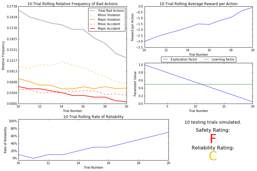
vs.plot_trials('sim_default-learning.csv')
Question 6
Using the visualization above that was produced from your default Q-Learning simulation, provide an analysis and make observations about the driving agent like in Question 3. Note that the simulation should have also produced the Q-table in a text file which can help you make observations about the agent’s learning. Some additional things you could consider:
- Are there any observations that are similar between the basic driving agent and the default Q-Learning agent?
- Approximately how many training trials did the driving agent require before testing? Does that number make sense given the epsilon-tolerance?
- Is the decaying function you implemented for $\epsilon$ (the exploration factor) accurately represented in the parameters panel?
- As the number of training trials increased, did the number of bad actions decrease? Did the average reward increase?
- How does the safety and reliability rating compare to the initial driving agent?
Answer:
The incidence of major and minor accidents are very similar between the no-learning and the Q-learning cases. There were approximately 19 training trials before beginning testing which, given an epsilon tolerance of 0.05, makes sense. As the number of training trials increased, the frequency of bad actions decreased and the average reward, although negative still, increased. These two observations are encouraging that the algorithm, thus far, is doing something positive. The reliability increases as the trial number increases, which is to be expected while learning. Safety, however, is very much a concern; the safety rating over the test trials was graded ‘F’.
Improve the Q-Learning Driving Agent
The third step to creating an optimized Q-Learning agent is to perform the optimization! Now that the Q-Learning algorithm is implemented and the driving agent is successfully learning, it’s necessary to tune settings and adjust learning paramaters so the driving agent learns both safety and efficiency. Typically this step will require a lot of trial and error, as some settings will invariably make the learning worse. One thing to keep in mind is the act of learning itself and the time that this takes: In theory, we could allow the agent to learn for an incredibly long amount of time; however, another goal of Q-Learning is to transition from experimenting with unlearned behavior to acting on learned behavior. For example, always allowing the agent to perform a random action during training, i.e. when $\epsilon = 1$ and never decays, will certainly make it learn, but never let it act. When improving on your Q-Learning implementation, consider the implications it creates and whether it is logistically sensible to make a particular adjustment.
Improved Q-Learning Simulation Results
To obtain results from the initial Q-Learning implementation, you will need to adjust the following flags and setup:
-
'enforce_deadline'- Set this toTrueto force the driving agent to capture whether it reaches the destination in time. -
'update_delay'- Set this to a small value (such as0.01) to reduce the time between steps in each trial. -
'log_metrics'- Set this toTrueto log the simluation results as a.csvfile and the Q-table as a.txtfile in/logs/. -
'learning'- Set this to'True'to tell the driving agent to use your Q-Learning implementation. -
'optimized'- Set this to'True'to tell the driving agent you are performing an optimized version of the Q-Learning implementation.
Additional flags that can be adjusted as part of optimizing the Q-Learning agent:
-
'n_test'- Set this to some positive number, previously 10, to perform that many testing trials. -
'alpha'- Set this to a real number between 0 - 1 to adjust the learning rate of the Q-Learning algorithm. -
'epsilon'- Set this to a real number between 0 - 1 to adjust the starting exploration factor of the Q-Learning algorithm. -
'tolerance'- set this to some small value larger than 0, default was 0.05, to set the epsilon threshold for testing.
Furthermore, use a decaying function of your choice for the exploration factor $\epsilon$. Note that whichever function you use, it must decay to 'tolerance' at a reasonable rate. The Q-Learning agent will not begin testing until this occurs. Some example decaying functions, where $t$, is the number of trials:
\(\epsilon = a^t, \textrm{for } 0 < a < 1 \hspace{50px}\epsilon = \frac{1}{t^2}\hspace{50px}\epsilon = e^{-at}, \textrm{for } 0 < a < 1 \hspace{50px} \epsilon = \cos(at), \textrm{for } 0 < a < 1\) You may also use a decaying function for the learning rate $\alpha$ if you so choose, however this is typically less common. If you do so, be sure that it adheres to the inequality $0 \leq \alpha \leq 1$.
If you have difficulty getting your implementation to work, try setting the 'verbose' flag to True to help debug. Flags that have been set here should be returned to their default setting when debugging. It is important that you understand what each flag does and how it affects the simulation!
Once you have successfully completed the improved Q-Learning simulation, run the code cell below to visualize the results. Note that log files are overwritten when identical simulations are run, so be careful with what log file is being loaded!
# Load the 'sim_improved-learning' file from the improved Q-Learning simulation
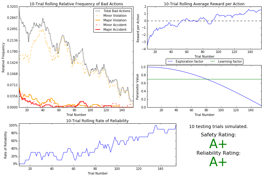
vs.plot_trials('sim_improved-learning.csv')
Question 7
Using the visualization above that was produced from your improved Q-Learning simulation, provide a final analysis and make observations about the improved driving agent like in Question 6. Questions you should answer:
- What decaying function was used for epsilon the exploration factor?
- Approximately how many training trials were needed for your agent before begining testing?
- What epsilon-tolerance and alpha learning rate did you use? Why did you use them?
- How much improvement was made with this Q-Learner when compared to the default Q-Learner from the previous section?
- Would you say that the Q-Learner results show that your driving agent successfully learned an appropriate policy?
- Are you satisfied with the safety and reliability ratings of the *Smartcab?*
Answer:
I chose the $\epsilon = \cos(at)$ decaying function with $a = 0.01$. The smartcab needed about 140 training trials before testing, based upon the ‘reward per action’ and ‘relative frequency’ metrics. However, training for about 20 more runs for additional refinement was performed. The epsilon tolerance used was 0.05 and the learning rate was $\alpha = 0.7$. These were the best values in terms of the previously mentioned metrics considered when performing multiple trials. The updated Q-learner displayed much lower relative frequency of bad actions 0.10 less, violations 0.10 aggregate, and a lower incidence of accidents, 0.04, when compared with the default. There is a net positive reward per action in the updated learner whereas there is still a net negative reward per action in the default. The reliability and safety scores show huge differences; the updated policy gets ‘A+’ scores for both, whereas the scores for the default are much less impressive. I would say that the agent learned an appropriate policy based on the exemplary scores displayed above. I am very satisfied with the safety and reliability ratings.
Define an Optimal Policy
Sometimes, the answer to the important question “what am I trying to get my agent to learn?” only has a theoretical answer and cannot be concretely described. Here, however, you can concretely define what it is the agent is trying to learn, and that is the U.S. right-of-way traffic laws. Since these laws are known information, you can further define, for each state the Smartcab is occupying, the optimal action for the driving agent based on these laws. In that case, we call the set of optimal state-action pairs an optimal policy. Hence, unlike some theoretical answers, it is clear whether the agent is acting “incorrectly” not only by the reward (penalty) it receives, but also by pure observation. If the agent drives through a red light, we both see it receive a negative reward but also know that it is not the correct behavior. This can be used to your advantage for verifying whether the policy your driving agent has learned is the correct one, or if it is a suboptimal policy.
Question 8
Provide a few examples, using the states you’ve defined, of what an optimal policy for this problem would look like. Afterwards, investigate the 'sim_improved-learning.txt' text file to see the results of your improved Q-Learning algorithm. For each state that has been recorded from the simulation, is the policy, the action with the highest value, correct for the given state? Are there any states where the policy is different than what would be expected from an optimal policy? Provide an example of a state and all state-action rewards recorded, and explain why it is the correct policy.
Answer:
Let’s consider the three states: (‘left’, (‘red’, ‘forward’, None)), (‘left’, (‘red’, ‘forward’, None)), and (‘left’, (‘green’, ‘forward’, ‘left’)). The first entry in the state vector is the next waypoint and the second entry is a 4-tuple made up of traffic light signal, oncoming car direction at intersection, left car action at intersection, and right car action at intersection.
The optimal policy for the first state would be no action (‘None’). Sitting at the red is required to avoid an accident
The optimal policy for the second state would again be no action. Either going straight or making a left turn would not only be a traffic violation, but would also be very unsafe in this particular state. Going right negatively impacts efficiency, but it is safe. The simulation gives the following for Q:
(‘left’, (‘red’, ‘forward’, None)) – forward : -6.63 – right : 0.60 – None : 1.44 – left : -6.74
This policy captures well the strategy discussed in the previous paragraph. I would expect that further learning would reduce the value for ‘right’ relative to the value for ‘None’.
The optimal policy for the third state, since waiting at a green light is more heavily penalized than going in the wrong direction, one only effects efficiency while the other violates traffic law, would be to go forward. Going straight or making a right turn would be safe, but negatively impact efficiency *i.e. a right turn should have lower Q than going straight due to the waypoint. Taking no action violates traffic laws and should be avoided. Making a left would cause an accident with the oncoming car going straight and violate traffic law. The simulation gives the following for Q:*
(‘left’, (‘green’, ‘forward’, ‘left’)) – forward : 0.00 – right : 0.41 – None : 0.00 – left : -13.80
The policy here is a right turn. While this is a legal action I would’ve expected the ‘forward’ Q to be greater than the Q score for ‘right’ due to efficiency concerns. Therefore, this policy at this state is clearly suboptimal.