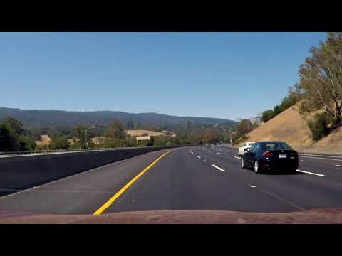
Single Shot Detection & Tracking

Abstract

A single shot detector is built to identify cars within a given video stream. The output of the detector is minimal bounding boxes around detected cars. Bounding box transients are smoothed using a Kalman filter tracker implemented in pixel space.

Outline

This project is broken into the following steps:

• Perform feature extraction on a given labeled training set of images, aka preprocessing
• Train a classifier
• Perform sliding-window search and use the trained classifier to detect vehicles in images.
• Run the full processing pipeline on a video stream and create a heat map of recurring detections frame by frame to reject outliers and follow detected vehicles.
• Estimate a bounding box for vehicles detected.

Here’s a link to the video that will be processed:

For all project materials, please see this GitHub repo.

Preprocessing

Histogram of Oriented Gradients

For object detection within images, Histogram of Oriented Gradients is a powerful technique. The gist of HOG is that object shape can be extracted from the distribution of intensity gradients or edge directions, hence the orientation piece. I’ll outline the steps below for implementing a HOG feature extraction for object detection.

The code for this step is contained in the function get_hog_features (or in lines 6 through 24 of the file called lesson_functions.py). The call to this function is in extract_features (lines 45-95 of lesson_functions.py). The function extract_features is called in the main routine (lines 41-46 in classify.py).

Before getting into the construction of feature vectors, though, some preliminary steps were taken:

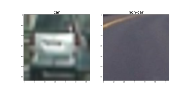
I started by reading in all the vehicle and non-vehicle images. Here is an example of one of each of the vehicle and non-vehicle classes:

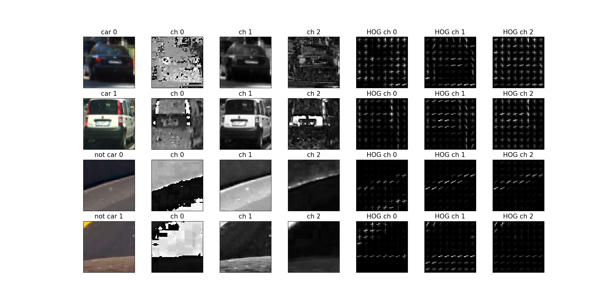
I then explored different color spaces and different skimage.feature.hog() parameters (orientations, pixels_per_cell, and cells_per_block). I grabbed random images (random since the paths were shuffled using the sklearn.model_selection.train_test_split function) from each of the two classes and displayed them to get a feel for what the skimage.feature.hog() output looks like.

Here is an example using the HLS color space and HOG parameters of orientations=9, pix_per_cell=(8, 8) and cells_per_block=(2, 2):

I tried various combinations of parameters and settled on those which, along with the chosen classifier, gave a large accuracy on both the training and validation sets. For me, I thought that accuracies within 1% of each other above 97% was sufficient. For the final parameter set chosen, see lines 28-37 in classify.py.

Training a Classifier

I trained a linear SVM using default parameters (see this). For the specific implementation, see lines 74-80 in classify.py. The linear SVM was chosen over higher-order kernel methods since it provided sufficient accuracy on both the training and validation data sets while minimizing classification time; about 98%.

Sliding Window Search

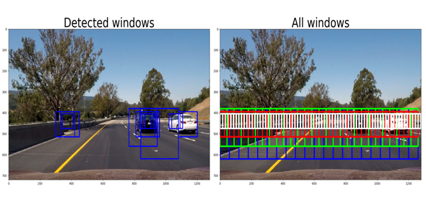
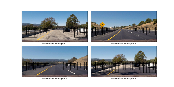
Since we only really care about vehicles below the horizon, I minimized the amount of y pixels to be searched over. After much trial-and-error, values were chosen that gave decent detection performance on images within the test_images directory (see line 52-58 of searcher.py in the search_all_scales function. The implementation of the sliding window search algorithm is contained within the slide_window function (see lines 101-143 in lesson_functions.py). The gist of the algorithm is to create windows based upon desired overlap and pixel positions and then append, and subsequently return, a list containing valid windows to search for detections across. This is the first part of the process. The second part is contained within the search_all_scales function within searcher.py (lines 47-76). In this routine, “hot” windows are identified by a call to search_windows, which uses the linear svm classifier trained previously to determine whether or not a car detection was made within that window. The definition of search_windows is in lesson_functions.py (lines 209-238). For an example of output on test images from this approach, see the following:

Putting it All Together

After trial over multiple scales, and different overlap ratios, I ultimately searched on 4 scales using HLS 3-channel HOG features plus spatially binned color and histograms of color in the feature vector. The feature vector was then scaled using sklearn.preprocessing.StandardScaler() (see lines 52-57 of classify.py) to ensure appropriate scaling. Here are some example images:

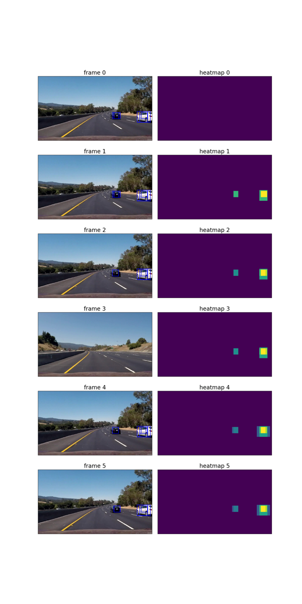
There are clearly some issues with false positives. To address these issues, I recorded the positions of positive detections in each frame of the video. From the positive detections I created a heatmap and then thresholded that map to identify vehicle positions. I then used scipy.ndimage.measurements.label() to identify individual blobs in the heatmap. Assuming each blob corresponded to a vehicle, I constructed bounding boxes to cover the area of each blob detected.

Here’s an example result showing the heatmap from a series of frames of video, the result of scipy.ndimage.measurements.label() and the bounding boxes then overlaid on a frame within the video:

IMPORTANT NOTE: I used the following commands, from within the project directory, to generate the heatmap directory and subsequent files needed for the plots below: mkdir heatmap; ffmpeg -i project_video.mp4 -r 60/1 heatmap/output%03d.jpg

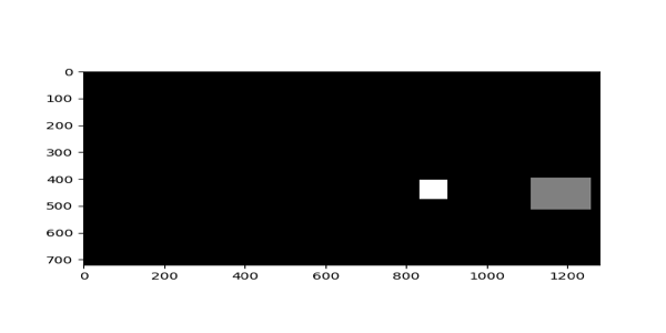
Here is the output of scipy.ndimage.measurements.label() on the integrated heatmap from all six frames:

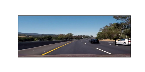
Here the resulting bounding boxes are drawn onto the last frame in the series:

After All the Postprocessing…

Below you’ll find a link to the processed video (minus the tracker):

Tracking

The detector performs reasonably well, but the bounding boxes are a little noisy. I next added a Kalman filter to smooth out the bounding boxes. The Kalman filter process model I chose, based upon how linear the motion of the vehicles seemed, is constant velocity with a constant aspect ratio. The constant aspect ratio seemed appropriate given that, as a vehicle moves towards the horizon, will scale smaller equally in both width and height.

There was also the problem of data association: How do I pick which measurement associates to which track from frame-to-frame? I chose a simple, greedy algorithm that picks the measurement-track pair that yields the smallest normalized-innovation-squared at the prediction step. This is a pretty typical approach.

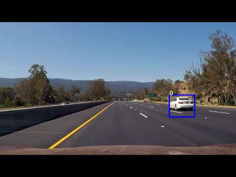
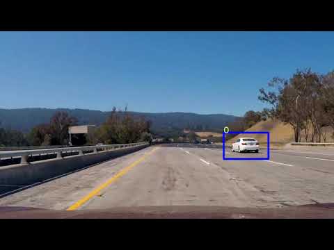
Here’s a link to the full pipeline; detection + tracker:

Concluding Remarks

There was a lot of trial-and-error trying to get decent performance on the videos; all tuning effort, after heatmap filtering, was focused on performance on the video. The results look pretty good.

To make the pipeline more robust, I would like to have more time to investigate additional features to add for classification. All things considered, performance was pretty good with a quite limited feature set.

From the video, it’s clear that that there are issues when two vehicles come within a single window search area. Individual vehicles are difficult to resolve in this case. Therefore, the pipeline will most likely have difficulty in high volume, crowded freeway and street traffic situations. There is a pretty good deep learning network architecture that handles such simulations well on GPUs with low computational overhead. I’ll write a shorter post about this when I have a chance. It’s pretty cool so stay tuned!