GitHub

Abstract

A full stack unmanned aerial vehicle (UAV) simulation is built using the starter project provided by Dr. Randy Beard, one of the coauthors of “Small Unmanned Aircraft: Theory and Practice. The starter project is a companion to the book that walks students through the incremental development of the simulation using end-of-chapter design projects. The culmination of my work is the result seen above: planning and executing a safe path through an urban environment using noisy sensor data and moderately gusty wind (over 10 feet/sec mean).

Building the UAV simulation, block-by-block

The UAV system architecture can be decomposed into blocks; see the diagram below:

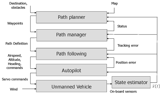
source: Beard and McLain, “Small Unmanned Aircraft: Theory and Practice”, Princeton University Press, 2012

The Unmanned Vehicle block

The “Unmanned Vehicle” block consists of the following elements necessary for simulation:

• Coordinate Frames (Chapter 2)
• Visualization (Chapter 2)
• Kinematics (Chapter 3)
• Dynamics (Chapter 4)

Coordinate Frames

Coordinate frames are important for all subsequent modeling and control methodologies to be discussed. The frames discussed in Chapter 2 define the angular and translational quantities that are used throughout the rest of the book.

Arguably, the most important relationship presented in Chapter 2 is the wind triangle:

What makes this relationship so important is that it can be used to infer the north, east, and down (inertial) components of the wind vector, \(\mathbf{w}\), from quantities that are measurable: ground speed (\(V_g\)), heading angle (\(\chi\)), flight path angle (\(\gamma\)), airspeed (\(V_a\)), yaw angle (\(\psi\)), and air-mass referenced flight path angle (\(\gamma_a\)).

All coordinate frames presented are Cartesian, which is appropriate for small aircraft that don’t need to account for the curvature or rotation of the Earth.

Visualization

The first design project is to create a graphical representation of a small, fixed wing aircraft. My solution is implemented in this commit. I chose values that were in proportion to relative lengths observed in the model from page 26 of the book. I defined the 3D (body-relative) coordinates of the vehicle’s vertices and then created a triangular mesh from these points. The ordering of the vertices in the mesh matters; vertices must be ordered according to the right-hand rule. Triangular elements of the mesh must have outward-facing normals: when you curl your fingers along the difference vector between pairs of vertices, your thumb should point away from the vehicle’s surface.

Kinematics

The six degree-of-freedom (DoF) equations-of-motion (EOM) for a rigid body moving through space are presented in Chapter 3. These EOM include translational and rotational motion in the presence of external forces and moments, respectively.

Dynamics

Chapter 4 presents the full balance of forces and moments for a fixed wing aircraft. Forces and moments applied to the body are a result of the following dynamic effectors:

• Aerodynamic surfaces (including control surfaces)
• Throttle (e.g., applied by a propeller)
• Gravity

The vehicle being modeled is “bank to turn”. In order to turn, the vehicle must first initiate a roll maneuver to change the orientation of the vehicle’s control surfaces.

The aerodynamic forces and moments are, to a large degree, matters of design: forces and moments scale linearly with air density (\(\rho\), which scales proportionally with altitude) and wing planform area (\(S\)), and quadratically with airspeed. The forces and moments are also linearly proportional to non-dimensional aerodynamic coefficients that can be linearized in Taylor expansions about a fixed point. Aircraft are normally designed such that they can achieve static stability; when the aircraft is perturbed away from a trim point (where forces and moments are in balance), the resulting aerodynamic forces and moments drive the vehicle back towards that same equilibrium. Control surfaces also affect the aerodynamics of the vehicle. As the name indicates, forces and moments arising from control surfaces are applied to drive the vehicle towards certain operational objectives, including:

• Altitude (\(h\))
• Airspeed (\(V_a\))
• Heading (\(\chi\))

The forces and moments of this chapter are separated into two channels: longitudinal and lateral.

The longitudinal dynamics consist of the lift and drag forces on the vehicle, as well as the pitching moment. These forces and moment are affected by control inputs from the throttle and elevator control surface, the body pitching rate, as well as the orientation of the vehicle’s velocity vector relative to wind (i.e., the angle-of-attack \(\alpha\)). Altitude and airspeed are consequences of the longitudinal forces and moments.

The lateral dynamics are a consequence of the rudder and aileron control inputs, the body roll and yaw rates, as well as the the orientation of the vehicle’s velocity vector relative to wind (i.e., the sideslip angle \(\beta\)). The vehicle’s heading is a consequence of the lateral forces and moments.

The Autopilot block

The “Autopilot” block is responsible for generating flight controls to stably achieve flight plan objectives for altitude, airspeed, and heading. Designing an autopilot, also called a flight controller, starts with creating reduced order models for the nonlinear dynamics of the vehicle. These models are presented in Chapter 5.

The methods described in the book separate the full 6DoF EOM into lateral and longitudinal channels. The lateral and longitudinal channels are then further simplified into representative linear models. These linear models can be used to design flight controllers with feedback for each channel using proportional-integral-derivative (PID) controllers. Chapter 6 describes an approach for implementing PID controllers for both the lateral and longitudinal channels so that objectives can be met. The approach requires state feedback be available. For the purpose of motivating the autopilot design, true state feedback is used. State feedback based on sensor measurements and an observer model is presented later in the book.

While decomposing the full EOM into channels is useful in simplifying controller design, the approach results in undesirable control coupling. As I describe in this post, other methods can be used that better account for this coupling. Two methods discussed in the post are Linear Quadratic Regulator (LQR) control and Total Energy Control System (TECS) control.

LQR control seeks to analytically compute a control command that minimizes a control objective. This control objective is a quadratically-weighted balance between system error and control effort and must be carefully chosen by the control designer. LQR is mathematically precise, however it suffers when there is significant modeling error. Sources of modeling error in LQR include system modeling errors (like from forces and moments), truncation error (when trying to linearize a highly nonlinear system), and unmodeled disturbances (such as wind gusts).

TECS control seeks to generate a control command that regulates the total energy (kinetic plus potential) of the aircraft while seeking to achieve the vehicle’s altitude, airspeed, and heading references. The TECS method proposed in the post is great because it better accounts for coupling between altitude and airspeed dynamics and because no linearization of the model is required. One drawback of this approach is that, when the vehicle encounters significant wind, an additional regulator (a PI controller in this case) must be added to remove steady-state errors in altitude and airspeed. These errors are a consequence of kinetic energy being a function of ground speed, not airspeed. Since airspeed is being regulated, a correction must be applied in addition to the TECS command. TECS is also fundamentally limited to longitudinal control since heading has no impact on the total energy of the system.

In the post, I showed that the LQR controller works well when implemented for both channels, however the TECS controller better decouples airspeed and altitude dynamics. To get the best of both LQR and TECS, I implemented a hybrid controller here. The results of this approach are shown below:

In the presence of moderate wind, the controller aggressively tracks step changes in its reference altitude, airspeed, and heading commands. The vehicle is clearly working hard to quickly eliminate errors and, in practice, such maneuvering is not necessary.

Because the PID controller is simpler to tune and performs reasonably well, I used it for the remainder of the design projects.

The State Estimator block

Chapter 7 presents models for various UAV sensors, including:

• Accelerometers
• Gyroscopes
• Altimeters (Static Pressure)
• Airspeed sensors (Dynamic Pressure)
• Global Positioning System (GPS)
• Magnetometers

Chapter 8 presents observer models to estimate the UAV’s state vector from sensor measurements. This state vector is then used as feedback to the autopilot.

As described in this post, I made a number of modifications to the method presented in Chapter 8, including

• The inclusion of the magnetometer heading estimate
• The addition of vertical plane GPS measurements
• The fusion of the altimeter and GPS altitude measurements into a unified altitude estimate
• The dynamic adjustment of the observer model’s process noise based on how well the model prediction agrees with measurements.

As shown below, the observer model tracks truth pretty well. This is especially notable considering there is no direct way of measuring wind using sensor estimates. Discrepancies are seen when a large step response in any reference input happens, but the estimates quickly converge back to the expected (i.e., true) values.

The Path Follower block

Having established in the previous design projects that it is possible to command step changes in the vehicle’s altitude, airspeed, and heading using only estimates for state feedback, getting the vehicle to follow desirable paths is now possible. Perhaps simplistically, paths can be modeled as lines or circles. Chapter 10 presents methods for tracking a line or a circle in the presence of moderate wind. “Tracking” a path in this context means driving the error between the current UAV position in inertial coordinates and a point on the path to zero. This error is sometimes referred to as “crosstrack error”. The system behavior in response to a commanded line path is shown below:

The plot above demonstrates how the vehicle manages its orientation to account for the effects of wind. If no wind were present, the vector between the nose and tail would be coincident with the linear path segment, which would mean zero angle-of-attack and sideslip angle.

The Path Manager block

The path management techniques in Chapter 11 describe ways of performing missions that fly through a set of prescribed waypoints. A waypoint is point in 3D space that an operator would like the vehicle to fly to. A waypoint may or may not include a desired heading to achieve along with the 3D point in space.

A path manager takes an input sequence of waypoints that an operator would like the vehicle to fly through. Internal to the path manager is a process for deconstructing waypoint sequences into line and circular arc segments so that vehicles can efficiently traverse paths between consecutive waypoints. The path manager also handles transitioning from the current target waypoint to the next when certain conditions are met. Three approaches to path management are presented in the chapter:

• Linear - waypoints are connected by linear path objectives
• Fillet - the transition from one waypoint to another follows a circle connecting adjacent waypoint linear segments
• Dubins - paths between consecutive waypoints are deconstructed into three segments - an arc, followed by a line, concluded by an arc

Of the three options presented, only the Dubins approach ensures that generated paths actually fly through each prescribed waypoint. The Dubins approach also provides an operator the ability to prescribe a desired heading at each waypoint. Neither of the first two approaches gives this ability. Below are the results for an example “Figure-8” mission using the Dubins approach:

The Path Planner block

The culmination of the book, in my opinion, is the presentation of material pertaining to path planning. Chapter 12 describes techniques for generating safe, i.e., collision-free, paths between starting and goal positions. These paths are simply a sequence of waypoints for which safe connecting paths are generated. Once planned, these waypoint sequences can be handed over to the path manager for execution. The results for the rapidly-exploring random tree (RRT) planner are shown at the beginning of this writeup.

Afterword: Target Tracking

I would have been fine if the authors had concluded the book with the chapter on path planning. However, as an added bonus, a chapter on target tracking and geolocation is presented. This is an important topic, so much so that I believe it should have been treated in a separate volume of this book so that it could be more thoroughly developed with respect to the following:

• Path planning - how do you generate safe paths, including some minimum safe standoff distance?
• Centering the target in the camera field-of-view (FoV)
• Estimating target motion in the image plane

Still, I thought this was a valuable chapter and I will refer back to it regularly. Below are the results from Chapter 13’s design project for pointing the camera at a target.

The error in estimating the state of the aircraft has clearly affects the position of the target in the image plane; the target is expected to be in the center of the FoV and it clearly is not. There are other issues as well, like the fact that even when the target is behind a building, the camera is still pointing at it.

Wrap-up

I learned a lot about fixed wing aircraft while working through the design projects from this book. The material is really interesting and the projects provide a fantastic way of reinforcing the lessons. I like that there are so many directions to which this material can be applied. Personally, I was most interested in flight controllers and state estimators when going through this book, so I focused a lot of my attention on the related chapters. If I were to go through this book again I would focus more on the later chapters. In particular, I would like to learn more about target-aware path planning.

Thanks for reading!